|
|
|
|
Visualization and Analysis of Quantum Chemical and Molecular Dynamics Data with VMD Part 2 |
|
4. Loading and Displaying Configurations and Trajectories
![]()
4.1. Loading a Single Geometry
![]()
4.2. Creating a Visualization
![]()
4.3. Saving and Re-using a Visualization
![]()
4.4. Viewing a Trajectory
![]()
4.5. How to Show Breaking and Formation of Bonds
![]()
4.6. Adding Graphics to a Visualization
![]()
![]() Part 1
Part 1
![]() Part 3
Part 3
![]() Start
Start
![]() Contents
Contents
There are several ways of how you may want to look at configurations generated by Single Point and MD calculations. The following sections will give you some examples on how to visualize single geometries, whole trajectories, Wannier centers, and (optionally) copies of the simulation unit cell, which can be very helpful for systems with periodic boundary conditions.
 The easiest way to load molecules from CPMD calculations into VMD
would be to load the GEOMETRY.xyz file that recent CPMD versions
(3.5.x and later) generate by default. Beginning with VMD version 1.8.2
CPMD style xyz files are supported. If you have an older version of VMD,
you have to first convert the file to a supported format, e.g. PDB, with
Babel
or Open Babel
(VMD has internal Babel support, if installed correctly).
The easiest way to load molecules from CPMD calculations into VMD
would be to load the GEOMETRY.xyz file that recent CPMD versions
(3.5.x and later) generate by default. Beginning with VMD version 1.8.2
CPMD style xyz files are supported. If you have an older version of VMD,
you have to first convert the file to a supported format, e.g. PDB, with
Babel
or Open Babel
(VMD has internal Babel support, if installed correctly).
For PWscf calculations you can use the scripts pwi2xsf.sh and/or pwo2xsf.sh to convert the respective input and output files to the xsf format, which is supported by VMD since version 1.8.3. Alternatively, you can use the simple pwscf2xyz.awk awk script to convert (some) PWscf output files to xyz format (this script may need some adjustments to support older/newer versions of PWscf). Please note, that the xsf format also usually contains the information of the supercell, which is not available for xyz files.
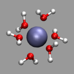
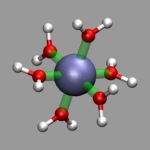
For the configuration on the left and the following examples, use the
file al-h2o_6.xyz. You can load this file
into VMD by just typing vmd al-h2o_6.xyz and you should see
something very similar to the picture on the left. In the next sections
we are trying to improve it a little bit.
 Once you have loaded a geometry into VMD, you can visualize it using a
single or multiple representations for all or a subset of the atoms.
The standard visualization method 'Lines' (see picture above) is usually
best suited to quickly look at a long trajectory or a very large
system. Also it does not need a very fast 3d-accelerated graphics
hardware, but for presentations you usually want to have something more
sophisticated. For example, in the picture on the left the water atoms
are selected by 'name H O' which is the short form of
'name H or name O' and visualized by
a 'CPK' representation while the aluminum is selected with
'name Al' and visualized by a 'VDW' representation
with a sphere size of 0.6. This way you can recognize the structure of
your configuration more clearly. More detailed explanations of this
procedure and examples of the various representations integrated into
VMD can be found in the excellent
VMD User's Guide
Once you have loaded a geometry into VMD, you can visualize it using a
single or multiple representations for all or a subset of the atoms.
The standard visualization method 'Lines' (see picture above) is usually
best suited to quickly look at a long trajectory or a very large
system. Also it does not need a very fast 3d-accelerated graphics
hardware, but for presentations you usually want to have something more
sophisticated. For example, in the picture on the left the water atoms
are selected by 'name H O' which is the short form of
'name H or name O' and visualized by
a 'CPK' representation while the aluminum is selected with
'name Al' and visualized by a 'VDW' representation
with a sphere size of 0.6. This way you can recognize the structure of
your configuration more clearly. More detailed explanations of this
procedure and examples of the various representations integrated into
VMD can be found in the excellent
VMD User's Guide
 If you have spent some time on a specific representation of your system,
you would usually like to somehow store that effort and reuse or improve
it later. For that you can use the File -> Save State...
dialog. You are asked to provide a filename (using the filename extension
.vmd is recommended) which will contain the VMD script code to
reproduce the current visualization. Since it is not an exact replay of
all your actions, it will sometimes fail to give the exact
same state, that you have saved, but usually it is pretty close.
If you have spent some time on a specific representation of your system,
you would usually like to somehow store that effort and reuse or improve
it later. For that you can use the File -> Save State...
dialog. You are asked to provide a filename (using the filename extension
.vmd is recommended) which will contain the VMD script code to
reproduce the current visualization. Since it is not an exact replay of
all your actions, it will sometimes fail to give the exact
same state, that you have saved, but usually it is pretty close.
 After you have saved a visualization you can reload it from the
File -> Load State... dialog or just run the script at VMD
startup e.g. with vmd -e saved_state.vmd. If you want to reuse
the visualiztion with a different coordinate or trajectory file, you
simply copy the the state file and modify it with a text editor (search
for the mol new statement(s)).
After you have saved a visualization you can reload it from the
File -> Load State... dialog or just run the script at VMD
startup e.g. with vmd -e saved_state.vmd. If you want to reuse
the visualiztion with a different coordinate or trajectory file, you
simply copy the the state file and modify it with a text editor (search
for the mol new statement(s)).
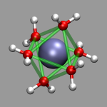
For the images in this section the visualization from the previous section, al-h2o_6.vmd, was loaded and then a 'Dynamic Bonds' representation was added to emphasize the octahedral arrangement of the water molecules (selection: 'name O or name Al', cutoff: 2.5, material: Transparent). The final visualization is also available for download: al-h2o_6-b.vmd. Also the selection 'name O' in combination with a cutoff of 3.0 can be used for a different way to show the octahedron.
For efficient working with VMD it is essential, that you understand how VMD processes the data. Trajectory data is in fact handled in multiple steps. First VMD reads the 'structure', i.e. it wants to know how many atoms of which type, with which bonds you want to display. If the bond information is missing in the file that was read in, it tries to guess the bonds via a distance search. This information will be applied for the whole trajectory, so the number or the ordering of the atoms must not change (thanks to the scripting capabilities of VMD, this limitation can be worked around to some degree). In the second step VMD wants to know the evolution of coordinates for each atom in the 'structure' during the trajectory. To achieve this with CPMD, you have several options: 1) You can set the flag TRAJECTORY XYZ in the &CPMD section of your CPMD input file and then get an additional file named TRAJEC.xyz which you can load into VMD similar to GEOMETRY.xyz. 2) You can use the CPMD trajectory format input plugin to read TRAJECTORY file(s) directly into VMD (supported from version 1.8.2 onward). For that you have to first load a GEOMETRY.xyz file to get the 'structure' information (TRAJECTORY files only contain coordinates, velocities and the time step number). And 3) you can convert the TRAJECTORY file(s) into xyz format, e.g. with the help of an external program, e.g. the perl script traj2xyz.pl
For PWscf the situation is a bit simpler: the xsf format is very flexible and also supports animations, so using pwo2xsf.sh converter should be sufficient. If you are using VMD version 1.8.2 or earlier and cannot or do not want to upgrade, you can also try the pwscf2xyz.awk script to convert the a PWscf output to the xyx format.
 Note that you can load several trajectory files on top of each other, so
you don't have to combine them first into a single file if you want to
look at a long trajectory, that has been simulated in parts. For large
trajectory files it is recommended that you activate the option Load all
at once before you click on the load button. Otherwise it can take
quite a long time to load the trajectory since VMD tries to run an
animation of the trajectory during the load process as soon as enough
data is available. If you have already created an elaborate
visualization scheme and your graphics hardware is not very fast,
this can get pretty bad. If you start from a saved
state script file, you should append waitfor all to all mol
new and mol addfile commands.
Note that you can load several trajectory files on top of each other, so
you don't have to combine them first into a single file if you want to
look at a long trajectory, that has been simulated in parts. For large
trajectory files it is recommended that you activate the option Load all
at once before you click on the load button. Otherwise it can take
quite a long time to load the trajectory since VMD tries to run an
animation of the trajectory during the load process as soon as enough
data is available. If you have already created an elaborate
visualization scheme and your graphics hardware is not very fast,
this can get pretty bad. If you start from a saved
state script file, you should append waitfor all to all mol
new and mol addfile commands.
One more tip: Since reading large text mode trajectories takes a lot of time, you could use the File -> Save Coordinates... dialog to save the read in coordinates in a binary trajectory format (e.g. DCD). This file will then load much faster (no more parsing required) and also usually takes up less diskspace. You only have to have an .xyz file for the first timestep to provide the structure information.
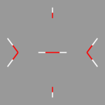
 One big problem for many programs to visualize ab initio MD trajectories
is how to handle formation or breaking of bonds. Programs that do this
dynamically (e.g.
Molden)
are usually not able to handle large trajectory files efficiently,
while other programs (e.g.
Molekel or the default
visualization of VMD) stick to the inital bond assignment. Recent
versions of VMD now offer a Dynamic Bonds representation, which
will recalculate the bonds every frame based on a given cutoff
distance. In combination with an additional VDW representation, you can
easily achieve a nice dynamical view of your simulation (see the small
animation on the left an example and compare it to the animation in the
previous section where only the CPK representation was used). If you
cannot get away with a single distance cutoff for all bonds, just use
several dynamic bond representations with different cutoffs on
individual groups of atoms.
One big problem for many programs to visualize ab initio MD trajectories
is how to handle formation or breaking of bonds. Programs that do this
dynamically (e.g.
Molden)
are usually not able to handle large trajectory files efficiently,
while other programs (e.g.
Molekel or the default
visualization of VMD) stick to the inital bond assignment. Recent
versions of VMD now offer a Dynamic Bonds representation, which
will recalculate the bonds every frame based on a given cutoff
distance. In combination with an additional VDW representation, you can
easily achieve a nice dynamical view of your simulation (see the small
animation on the left an example and compare it to the animation in the
previous section where only the CPK representation was used). If you
cannot get away with a single distance cutoff for all bonds, just use
several dynamic bond representations with different cutoffs on
individual groups of atoms.
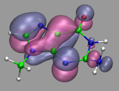
If your trajectory includes Wannier centers, the distance based bond selection will produce strange results. You could use the selections "not name X" for the atom representations and "name X" for the Wannier centers (looks pretty cool, if you use the Glass material and a VDW representation for the 'Wannier-atoms'. See the next chapter for some examples).
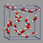
 For simulations with periodic boundary conditions it is frequently very
helpful to show the actual boundaries of the unit cell employed. For
that VMD gives you access to several graphics primitives that can be
added to a loaded molecule. This graphics primitives are drawn in the
molecule local coordinate system and so they moved, rotated, and resized
with all the representations belonging to that molecule. For the
following example we need the custom command
draw_cubic_unitcell
installed. After loading the trajectory from the files
32h2o_h3op.xyz and 32h2o_h3op.dcd we want to
mark the center of the simulation cell with a small yello ball and
then show the unitcell itself. With an edgelength of 9.956 Angstrom,
you have to give the following commands:
For simulations with periodic boundary conditions it is frequently very
helpful to show the actual boundaries of the unit cell employed. For
that VMD gives you access to several graphics primitives that can be
added to a loaded molecule. This graphics primitives are drawn in the
molecule local coordinate system and so they moved, rotated, and resized
with all the representations belonging to that molecule. For the
following example we need the custom command
draw_cubic_unitcell
installed. After loading the trajectory from the files
32h2o_h3op.xyz and 32h2o_h3op.dcd we want to
mark the center of the simulation cell with a small yello ball and
then show the unitcell itself. With an edgelength of 9.956 Angstrom,
you have to give the following commands:
# put a small yellow ball in the center of the box
draw color yellow
draw sphere {0 0 0} radius 0.25 resolution 20
# add simulation cell object
draw_cubic_unitcell 9.956
|
Full Table of Contents
![]()
1. Introduction
1.1. About this Tutorial
1.2. About the Programs
1.3. Notes
1.4. Citation / Bookmark
1.5. Recent Changes
2. Table of Contents
3. Preparation and Installation Issues
3.1. Customizing the VMD Setup
3.2. Predefining Additional Items
3.3. Extending the Script and Plugin Search Path
4. Loading and Displaying Configurations and Trajectories
4.1. Loading a Single Geometry
4.2. Creating a Visualization
4.3. Saving and Re-using a Visualization
4.4. Viewing a Trajectory
4.5. How to Show Breaking and Formation of Bonds
4.6. Adding Graphics to a Visualization
5. Adding Dynamic Graphics to a Trajectory
5.1. Adding a Progress Bar for the Elapsed Time
5.2. Display the Total Dipole Moment of the Simulation Cell
5.3. Visualizing Changing Atom Properties with Color
5.4. Modify an Atom Property Dynamically from an External File
6. Dynamic Atom Selection
6.1. Display a Changing Number of Molecules
6.2. Keeping Atoms or a Molecule in the Center and Aligned
6.3. Modify a Selection During a Trajectory
6.4. Using the User Field for Computed Selections
6.5. Tracing a Dynamic Property
7. Visualizing Volumetric Data from Cube-Files
7.1. Electron Density and Electrostatic Potential
7.2. Canonical and Localized Orbitals
7.3. Electron Localization Function (ELF)
7.4. Manipulation of Cube Files / Response to an External Potential
7.5. Bulk Systems
7.6. Animations with Isosurfaces
7.7. Volumetric data from Gaussian
8. Using Data Processing to Tailor Data for VMD
8.1. Visualizing Path-Integral Trajectories
8.2. Extracting the Geometry Information from old CPMD Output Files
8.3. Removing Unneeded Parts From a Cube File
8.4. Extract Some Coordinates with Bounding Box Information
8.5. Creating 3d-Ramachandran Histograms
9. Misc Tips and Tricks
9.1. Collected 'draw' Extensions
9.2. Using a Different Default Visualization
9.3. Changing the Default vdW Radii
9.4. Reloading the Current Trajectory
9.5. Visualize a Trajectory With a Changing Number of Atoms or Bonds
9.6. Set the Unit Cell Information for a Whole Trajectory
9.7. Directly Print the Current Visualization
9.8. Transferring a Visualization from a Molecule to Others
9.9. Adding a TCL-Plugin to the Extensions Menu
9.10. Turn Off Output in Analysis Scripts
9.11. Automatically Turn on TCL mode in (X)Emacs for .vmd Files
10. Credits
11. Downloads
12. Script distribution policy
|
|
|
||
|
|||