|
|
|
|
Visualization and Analysis of Quantum Chemical and Molecular Dynamics Data with VMD Part 5 |
|
7. Visualizing Volumetric Data from Cube-Files
![]()
7.1. Electron Density and Electrostatic Potential
![]()
7.2. Canonical and Localized Orbitals
![]()
7.3. Electron Localization Function (ELF)
![]()
7.4. Manipulation of Cube Files / Response to an External Potential
![]()
7.5. Bulk Systems
![]()
7.6. Animations with Isosurfaces
![]()
7.7. Volumetric data from Gaussian
![]()
![]() Part 4
Part 4
![]() Part 6
Part 6
![]() Start
Start
![]() Contents
Contents
Apart from calculating trajectories various volumetric properties can be calculated with the CPMD program: e.g. electron densities, spin densities, electrostatic potentials, electron localization functions (ELF), localized and canonical (occupied) orbitals. This data can be visualized with VMD via the Gaussian cube file format. Beginning with version 1.8.2 VMD fully supports reading atom coordinates and volumetric data in the cube file format. Please note that some of the examples need a very recent CPMD version (3.9.1 or newer) to work properly, as i found and fixed a few cubefile related bugs while creating this part of the tutorial (the same goes for the cpmd2cube program, a patch relative to the latest released version from cpmd.org is available on request). VMD version 1.8.3 and CPMD version 3.9.2 as well as the cpmd2cube version relased with it contain additional improvements, mainly for handling non-orthogonal supercells.
For some of the aforementioned properties cube file can be directly generated from cpmd, the rest is written in a native format which can be converted into a cube file with the help of the cpmd2cube program (available at the download area of http://www.cpmd.org). Since the CPMD manual is not very detailed about these tasks, the following section will give a few CPMD input file examples alongside the suggestions for visualizations.
To proceed with the following examples, we first need a fully converged wavefunction. This example input will generated that for an isolated water molecule in the gas phase:
 |
| |||
|
||||
|
By adding the keywords RHOOUT and ELECTROSTATIC POTENTIAL the electron density and the electrostatic potential will be written to files named DENSITY and ELPOT, respectively, at the end of the wavefunction optimization. Note the rather high cutoff of 120ryd which is not really required, but helps to get smooth surfaces. Since we want to re-use this restart file as base for further calculations, please rename it from RESTART.1 to RESTART. With RESTART WAVEFUNCTION COORDINATES (Note: no LATEST) all further calculation will always read in this 'high quality' restart and it will not be overwritten. Finally we need to convert the two volumetric files to cube files by:
cpmd2cube.x -o h2o-dens -dens DENSITY cpmd2cube.x -o h2o-pot -dens ELPOT |
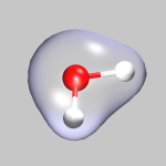
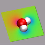
To visualize volumetric data in VMD you currently have two options: Isosurfaces and Volume Slices. The two images in the top left of this section give an example for both styles. The upper image shows in addition to a CPK model of the water molecule an isosurface of the electron density (for ρ = 0.05), the lower image a volume slice through the electrostatic potential (for y = 0.5). The CPMD input (h2o-dens-pot.in), the pseudopotential files (O_MT_PBE, H_MT_PBE), the resulting cube files (h2o-dens.cube, h2o-pot.cube) and a combined VMD script file (h2o-dens-pot.vmd) are available for download, so that you can experiment with it.
VMD version 1.8.3 introduces the Volume coloring method (for OpenGL implementations that support it), which can be used to colorcode the surface by the value of the electrostatic potential at the position of the surface, i.e. color-map the electrostatic potential to the surface. The value range of the colormap can be adjusted via the Color Scale Data Range fields in the Trajectory tab of the Isosurface representation. Note: that for a 'properly symmetric' behavior the electrostatic potential from CPMD calculations needs to be corrected, e.g. via the trimcube utility. Downloadable example files: h2o-dens.cube, h2o-pot-norm.cube, and h2o-pot-map.vmd.
 To calculate the canonical (i.e. projected to an atomic basis set)
and localized orbitals for our water molecule we need to do a properties
calculation starting from the previously generated
wavefunction. Both sets of orbitals can be calculated individually as
well as simultaneously (as done here). Note that when calculating
orbital cube files, especially for localized orbitals, the default cube
files contain a lot of unneeded data, so that using the
trimcube
utility, or the -trim
option to cpmd2cube is highly recommended to save disk space and
reduce the memory requirements of VMD.
To calculate the canonical (i.e. projected to an atomic basis set)
and localized orbitals for our water molecule we need to do a properties
calculation starting from the previously generated
wavefunction. Both sets of orbitals can be calculated individually as
well as simultaneously (as done here). Note that when calculating
orbital cube files, especially for localized orbitals, the default cube
files contain a lot of unneeded data, so that using the
trimcube
utility, or the -trim
option to cpmd2cube is highly recommended to save disk space and
reduce the memory requirements of VMD.
For the localized orbitals the keywords LOCALIZE and WANNIER WFNOUT are required. This generates a series of files with the names WANNIER_*.* which have to be converted to cube format with cpmd2cube.x -o h2o-local WANNIER_1.1. Note that you must not use the -dens option here.
For the projected orbitals the CUBEFILE ORBITALS keyword (plus the two additional lines specifying how many and which orbitals shall be written) is required. This will generate a series of cube files with the names PSI.*.cube, that can be read into VMD directly.
Alltogether the first part of the CPMD input now contains:
&CPMD PROPERTIES RESTART WAVEFUNCTION COORDINATES WANNIER WFNOUT ALL &END &PROP LOCALIZE CUBEFILE ORBITALS HALFMESH 4 1 2 3 4 &END |
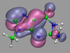
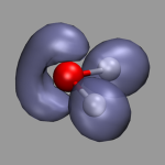
The picture on the left demonstrates the localized orbitals. Here all cube files have been read in on top of each other and visualized with an isosurface (blue for the lone pairs, green for the OH-bonds). The picture on the right shows the HOMO of the water molecule. Here the two different phases are visualized by creating two repesentations from the same data set and just using isovalues with opposite sign for each of them. The input and cube files used in this section are: h2o-orbs.in, h2o-local-1.cube, h2o-local-2.cube, h2o-local-3.cube, h2o-local-4.cube, h2o-orbs-local.vmd, h2o-homo.cube, and h2o-homo.vmd.
 The electron localization function (ELF) is a tool to describe chemical
bonding. It provides an alternative look into chemical bonding and
complements the picture gained by looking at the densities and orbitals.
The correlation between ELF and chemical bonding is a
topological and not an energetical one. So ELF can be said to represent
the organization of chemical bonding in direct space. Chemical
information can be obtained from ELF attractors taking the other
topological elements into account as well. The attractors can be attributed to
bonds, lone pairs, atomic shells and other elements of chemical bonding.
For more details please consult the ELF homepage at
http://www.cpfs.mpg.de/ELF/.
The electron localization function (ELF) is a tool to describe chemical
bonding. It provides an alternative look into chemical bonding and
complements the picture gained by looking at the densities and orbitals.
The correlation between ELF and chemical bonding is a
topological and not an energetical one. So ELF can be said to represent
the organization of chemical bonding in direct space. Chemical
information can be obtained from ELF attractors taking the other
topological elements into account as well. The attractors can be attributed to
bonds, lone pairs, atomic shells and other elements of chemical bonding.
For more details please consult the ELF homepage at
http://www.cpfs.mpg.de/ELF/.
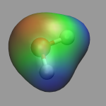
To calculate ELF with CPMD we need to add the keyword ELF PARAMETER to the &CPMD section of our input file. The resulting file named ELF is a density file similar to DENSITY and has to be converted to cube format with cpmd2cube. The picture on the left shows the ELF of our water example with an isovalue of 0.85. When increasing this value you can see, that the two lone pairs of the water are only partially localized. The relevant downloadable files are: h2o-elf.in, h2o-elf.cube, and h2o-elf.vmd.
Sometimes you need to postprocess the cube files, e.g. by calculating the difference between to densities. This can be done with the cubman utility from the Gaussian software suite. In this example we want to visualize the response of the a water molecule to an external potential perpendicular to the H-O-H plane.
For this purpose we first create an electron density cube file from the RESTART file of the previous examples with a simple properties job (cf. h2o-dens-nopot.in). The resulting file RHO_TOT.cube is renamed to h2o-nopot-dens.cube.
Now we need to create an unformatted fortran data file (extpot.unfo.grid) with the external potential on the grid points of the real space mesh of the CPMD job. In the current example this is a 80x80x80 grid so the fortran file has to use the same grid (e.g. in mkextpot.f). We now create a new wavefunction with the keyword EXTERNAL POTENTIAL (h2o-extpot.in), create another density cube file, and rename it to h2o-extpot-dens.cube.
Finally we use the cubman utility (see below for an example) to create
die difference of the two densities
(h2o-extpot-resp.cube) and visualize it. Here is a snapshot
of the interactive dialog.
# cpmd-vmd/files> cubman Action [Add, Copy, Difference, Properties, SUbtract, SCale]? su First input? h2o-nopot-dens.cube Is it formatted [no,yes,old]? yes Opened special file h2o-nopot-dens.cube. Second input? h2o-extpot-dens.cube Is it formatted [no,yes,old]? yes Opened special file h2o-extpot-dens.cube. Output file? h2o-extpot-resp.cube Should it be formatted [no,yes,old]? yes Opened special file h2o-extpot-resp.cube. |
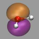
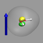
The image on the left shows the result. The arrow illustrates the direction of the electrostatic field represented by the external potential and the two colored isosurfaced show areas of reduced (green) and increased (yellow) electron density, the transparent isosurface represents the total electron density. The formation of an induced dipole moment in the water molecule is clearly visible. The figure was created with the VMD script h2o-extpot-resp.vmd.
 |
| (click here or on the image to view a larger version) |
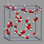
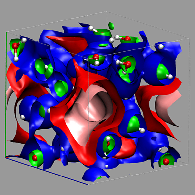
Creating and visualizing volumetric data is not restricted to isolated molecules, but can also be used for bulk systems, for example a bulk water system. Occasionally you have to make sure, that the cube file is properly centered and that all atoms are inside the density/simulation box. The command lines to get the cube files used here were:
cpmd2cube.x -o h2o-dens -inbox -center -dens DENSITY cpmd2cube.x -o h2o-elpot -inbox -center -dens ELPOT |
After visualizing the water molecules you can add one or more isosurface representations in order to display different isosurfaces from the same data set: blue (= negative electrostatic potential), red (= same value only positive), pink (=even more positive isovalue), and green (= electron density). Again the full saved state and the data file are available for download with the filenames h2o-cube.vmd, h2o-dens.cube, and h2o-elpot.cube.
 |
| (click here or on the image to view a larger version) |
With the help of a little bit of VMD scripting we can also do an animation with volumetric data, where the the isosurface is changed in each frame. In the present example, we have a simulation, in which a hydrogen molecule is shot at a double layer of gold atoms with very high velocity. We then need a cube file for each frame, that should be animated, therefor we need to instruct the CPMD program to write a (different) restart for each of these frames. This is done by using the STORE and RESTFILE keywords in the CPMD input file (for this example STORE was set to 20 and RESTFILE to 500 with a TIMESTEP of 2 a.u.). Now during the simulation (which should not exceed 10000 steps), a new restart is written every 20 steps.
The next step is to convert all of these restarts into cube files. This can done by doing one step of wavefunction optimization and using the keyword RHOOUT to write a DENSITY file, which then can be converted into a cube file with cpmd2cube.x. The first part of the CPMD input thus is:
&CPMD OPTIMIZE WAVEFUNCTION RESTART WAVEFUNCTION COORDINATES MAXSTEP 1 RHOOUT &END |
The conversion can be automated with:
for s in `seq 1 25` do \ rm -f RESTART ln -s RESTART.$s RESTART && ./cpmd.x au-dens.in && ./cpmd2cube.x -rho -o au-dens-$s DENSITY done |
We now load all those cube files in the correct order into VMD and create a visualization including an isosurface. To switch the volumetric data set during the animation, we write a small tcl procedure, that updates the representation and hook it into the animation loop by tracing vmd_frame. To make this as transparent as possible, we record the molecule id and the (unique) representation name of the isosurface in question in two global variables.
set updmol [mol new {au-dens-0.cube} type cube waitfor all]
...
set updrep [mol repname top 3]
...

proc update_iso {args} {
    global updmol
    global updrep

    set repid [mol repindex $updmol $updrep]
    if {$repid < 0} { return }

    set frame [molinfo $updmol get frame]
    lassign [molinfo $updmol get "{rep $repid}"] rep
    mol representation [lreplace $rep 2 2 $frame]
    mol modrep $repid $updmol
}

trace variable vmd_frame(0) w update_iso
|
There is one drawback: you have to know, which index the isosurface visualization has. But that is easily done (if you can count and remember, that the first representation id is 0), since you start from a script anyways. Any subsequent changes to the representations should be transparent to the script. You can download the full VMD script au-iso.vmd, and an archive with the cubefiles au-dens-cube.tar.gz (25MB).
In this section we take a small detour and discuss the visualization of volumetric outputs generated with the Gaussian electronic structure program. Since the cube file format was originally used in Gaussian visualizations like shown above are not restricted to CPMD calculations. The following are a few examples for using the Gaussian program, but this should be adaptable to other electron structure programs as well.
 The most convenient way of creating cube files from a
gaussian calculation is to use the cubegen and cubman
programs. Prerequisite is that you have saved a checkpoint file from
your calculation by adding a %Chk=filename.chk statement to
the header of your gaussian input file. The (binary) checkpoint file
needs to be converted into a formatted file using the formchk
utility (formchk filename.chk will produce the file
filename.fchk).
The most convenient way of creating cube files from a
gaussian calculation is to use the cubegen and cubman
programs. Prerequisite is that you have saved a checkpoint file from
your calculation by adding a %Chk=filename.chk statement to
the header of your gaussian input file. The (binary) checkpoint file
needs to be converted into a formatted file using the formchk
utility (formchk filename.chk will produce the file
filename.fchk).
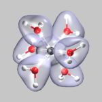
After these preparations we can finally start to generate some useful
cube files. We start with the electron density of a chromium-(III)-ion
surrounded by 6 water molecules (top left). This was created from the
formatted checkpoint file using the command:
cubegen 0 Density=scf cr-h2o_6-dubl.fchk
cr-h2o_6-dens-dubl.cube 60
For visualizing the density a single isosurface representation (after
visualizing the atoms itself) with a small positive isovalue, e.g. 0.05,
is sufficient (cr-h2o_6-dens.vmd).
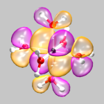 The next example shows orbital number 40
(the third highest occupied orbital) from the same calculation. Here
the command to create the cube file was:
cubegen 0 MO=40 cr-h2o_6-dubl.fchk
cr-h2o_6-orb-40.cube 60
For this visualization two isosurface representations are needed now,
one for positive and one for negative values (here: 0.01 and -0.01,
cr-h2o_6-orb-40.vmd).
If you want to show multiple different orbitals, you can either load
several of these single orbital cube files simultaneously, or create
a multi-orbital cube file by running a gaussian cube job (see the
gaussian manual on how to do it). VMD can load these multiple orbital
files as well as multiple cube file on top of each other and will
let you select the individual volumetric data sets in a pop-up menu
for the graphical representation menu.
The next example shows orbital number 40
(the third highest occupied orbital) from the same calculation. Here
the command to create the cube file was:
cubegen 0 MO=40 cr-h2o_6-dubl.fchk
cr-h2o_6-orb-40.cube 60
For this visualization two isosurface representations are needed now,
one for positive and one for negative values (here: 0.01 and -0.01,
cr-h2o_6-orb-40.vmd).
If you want to show multiple different orbitals, you can either load
several of these single orbital cube files simultaneously, or create
a multi-orbital cube file by running a gaussian cube job (see the
gaussian manual on how to do it). VMD can load these multiple orbital
files as well as multiple cube file on top of each other and will
let you select the individual volumetric data sets in a pop-up menu
for the graphical representation menu.
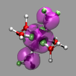
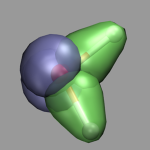
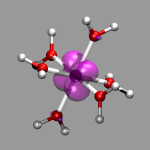 The final example shows the location of unpaired electrons
by calculating the difference between alpha- and
beta-electron spin density. For this two open shell Hartree-Fock
calculations were performed (one for the dublett state and one for the
quartett state), density cube files created and then the density
difference calculated by running cubman in subtract
mode on both cube files and thus creating a third cube file
(cr-h2o_6-dens-diff.cube). You can see the the single
unpaired electron in the dublett state is confined to a Chromium
d-orbital, whereas the three unpaired electrons of the quartett state
are rather delocalized.
The final example shows the location of unpaired electrons
by calculating the difference between alpha- and
beta-electron spin density. For this two open shell Hartree-Fock
calculations were performed (one for the dublett state and one for the
quartett state), density cube files created and then the density
difference calculated by running cubman in subtract
mode on both cube files and thus creating a third cube file
(cr-h2o_6-dens-diff.cube). You can see the the single
unpaired electron in the dublett state is confined to a Chromium
d-orbital, whereas the three unpaired electrons of the quartett state
are rather delocalized.
Full Table of Contents
![]()
1. Introduction
1.1. About this Tutorial
1.2. About the Programs
1.3. Notes
1.4. Citation / Bookmark
1.5. Recent Changes
2. Table of Contents
3. Preparation and Installation Issues
3.1. Customizing the VMD Setup
3.2. Predefining Additional Items
3.3. Extending the Script and Plugin Search Path
4. Loading and Displaying Configurations and Trajectories
4.1. Loading a Single Geometry
4.2. Creating a Visualization
4.3. Saving and Re-using a Visualization
4.4. Viewing a Trajectory
4.5. How to Show Breaking and Formation of Bonds
4.6. Adding Graphics to a Visualization
5. Adding Dynamic Graphics to a Trajectory
5.1. Adding a Progress Bar for the Elapsed Time
5.2. Display the Total Dipole Moment of the Simulation Cell
5.3. Visualizing Changing Atom Properties with Color
5.4. Modify an Atom Property Dynamically from an External File
6. Dynamic Atom Selection
6.1. Display a Changing Number of Molecules
6.2. Keeping Atoms or a Molecule in the Center and Aligned
6.3. Modify a Selection During a Trajectory
6.4. Using the User Field for Computed Selections
6.5. Tracing a Dynamic Property
7. Visualizing Volumetric Data from Cube-Files
7.1. Electron Density and Electrostatic Potential
7.2. Canonical and Localized Orbitals
7.3. Electron Localization Function (ELF)
7.4. Manipulation of Cube Files / Response to an External Potential
7.5. Bulk Systems
7.6. Animations with Isosurfaces
7.7. Volumetric data from Gaussian
8. Using Data Processing to Tailor Data for VMD
8.1. Visualizing Path-Integral Trajectories
8.2. Extracting the Geometry Information from old CPMD Output Files
8.3. Removing Unneeded Parts From a Cube File
8.4. Extract Some Coordinates with Bounding Box Information
8.5. Creating 3d-Ramachandran Histograms
9. Misc Tips and Tricks
9.1. Collected 'draw' Extensions
9.2. Using a Different Default Visualization
9.3. Changing the Default vdW Radii
9.4. Reloading the Current Trajectory
9.5. Visualize a Trajectory With a Changing Number of Atoms or Bonds
9.6. Set the Unit Cell Information for a Whole Trajectory
9.7. Directly Print the Current Visualization
9.8. Transferring a Visualization from a Molecule to Others
9.9. Adding a TCL-Plugin to the Extensions Menu
9.10. Turn Off Output in Analysis Scripts
9.11. Automatically Turn on TCL mode in (X)Emacs for .vmd Files
10. Credits
11. Downloads
12. Script distribution policy
|
|
|
||
|
|||