|
|
|
|
Visualization and Analysis of Quantum Chemical and Molecular Dynamics Data with VMD Part 3 |
|
5. Adding Dynamic Graphics to a Trajectory
![]()
5.1. Adding a Progress Bar for the Elapsed Time
![]()
5.2. Display the Total Dipole Moment of the Simulation Cell
![]()
5.3. Visualizing Changing Atom Properties with Color
![]()
5.4. Modify an Atom Property Dynamically from an External File
![]()
![]() Part 2
Part 2
![]() Part 4
Part 4
![]() Start
Start
![]() Contents
Contents
Sometimes you want to draw additional graphics the screen that show how some properties change during a trajectory. VMD offers you access to graphic primitves like lines, spheres, cylinders, cones, trangles and text with which you can add graphical elements to your molecule. To make these change with the evolution of the trajectory you can use the powerful Tcl variable tracing mechanism. In this case you want to trace the variable vmd_frame(). The following sections will give a few examples. The strategy is always the same:
5.1. Adding a Progress Bar for the Elapsed Time
 Although VMD shows the current frame number in the main window,
it is sometimes nicer to have an indicator of the elapsed
time in the visualization window. One big problem is, that the
progress indicator should stay fixed, even if the molecule itself
is rotated. As described above, usually you 'draw' in the coordinate
system of the molecule and so the added graphics would rotate with
the visualize molecule. This problem is avoided by creating an (empty)
stub molecule (by calling mol new without a file name),
fixing the position of that 'molecule' in the global coordinate system,
and adding the time bar graphics to the fixed 'molecule'. This is done
by the script function
display_time_bar.
Although VMD shows the current frame number in the main window,
it is sometimes nicer to have an indicator of the elapsed
time in the visualization window. One big problem is, that the
progress indicator should stay fixed, even if the molecule itself
is rotated. As described above, usually you 'draw' in the coordinate
system of the molecule and so the added graphics would rotate with
the visualize molecule. This problem is avoided by creating an (empty)
stub molecule (by calling mol new without a file name),
fixing the position of that 'molecule' in the global coordinate system,
and adding the time bar graphics to the fixed 'molecule'. This is done
by the script function
display_time_bar.
After you have loaded the trajectory from the files
zundel.xyz and zundel.dcd
and created a nice representation you run the following code:
# function to draw the time bar with the required options
proc do_time {args} {
# see source for explanations of the options
   display_time_bar 1.0 50.0 "fs" 0
}

# connect do_time to vmd_frame
trace variable vmd_frame(0) w do_time

# go back to the start of the trajectory
animate goto start
|
Now you can animate the trajectory as you like and the red line in the time bar will always the display the current time of the simulation. You can also move the mouse and the time display should stay fixed. The file zundel-time.vmd contains all the commands. You need to have the display_time_bar.tcl file installed properly to make this work. Alternatively you can copy the file to the current directory and add the command source display_time_bar.tcl to the .vmd script (or execute it manually) before you define do_time.
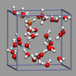
 For this example some external data needs to be read in. In this case
we use the corresponding data from the DIPOLE file created by
a CPMD simulation. By executing
For this example some external data needs to be read in. In this case
we use the corresponding data from the DIPOLE file created by
a CPMD simulation. By executing
awk '{ print $2, $3, $4; }' DIPOLE > zundel.dip
|
we can extract the current total diplol moment of the simulation cell
to zundel.dip.
We also need to have the following
commands installed
:
center_of_mass and
vmd_draw_vector.
Now we have to load the trajectory again and then execute
the following code:
# define function to (re-)draw the dipole vector
proc do_dipdraw {args} {
    # dipdata has the center and the direction/lenght of the vector
    # dipgraph has the indices of the vector graphic elements
    global dipdata dipgraph
    set molid 0
    set frame [molinfo $molid get frame]
    if {[info exists dipdata($frame)]} then {
        if {[info exists dipgraph]} then {
            foreach g $dipgraph {
              graphics $molid delete $g
            }
        }
        graphics $molid color yellow
        lassign $dipdata($frame) cnt vec
        #                                             scaling  res   radius
        set dipgraph [vmd_draw_vector $molid $cnt $vec 100000.0  10   0.08]
    }
}

# read in the dipole data from file
set dip [open "zundel.dip" r]
# define selection to calculate the center of mass
set sel [atomselect 0 "not name X"]
set n [molinfo 0 get numframes]
for {set i 0} {$i < $n} {incr i} {
    # advance selection to the current frame and update.
    $sel frame $n
    $sel update
    set dipdata($i) [list [center_of_mass $sel] [gets $dip]]
}
close $dip

# connect to vmd_frame
trace variable vmd_frame(0) w do_dipdraw
animate goto 0
|
Again the whole vmd script file is also available under the name
zundel-dip.vmd.
Of course, you can combine the time bar with the dipole vector display.
A vmd script file to do that is available under the name
zundel-all.vmd
NOTE:
for this simple example to work, the trajectory and the
dipole file have to be written with the same frequency.
 This example shows two C60 molecules colliding at high
temperature (500K). We utilize the 'user' field of the atom trajectory
data to store the distance of each atom from the center of mass of its
C60 molecule for each frame as a measure of the
deformation. This parameter is precomputed for the whole trajectory (so
this is extremely useful for expensive calculations)
and the coloring scheme 'User' is then used to display
the results (red is closer, green is normal, blue is further away).
Again we load the trajectory (bucky.xyz and
bucky.dcd) in the regular way, visualize the Atoms as VDW
spheres and Dynamic Bonds. To compute and store the distances we create
a selections for each molecule and use the integrated vector operations
of VMD. Note that a selection always returns a list of lists, so that
when requesting {x y z} for the selection we directly get the
individual vectors (=coordinate lists) stored into $c which
can be directly used for the vector math. To store the result, we then
have to provide a list of values for each atom in the selection. Here
is the final code:
This example shows two C60 molecules colliding at high
temperature (500K). We utilize the 'user' field of the atom trajectory
data to store the distance of each atom from the center of mass of its
C60 molecule for each frame as a measure of the
deformation. This parameter is precomputed for the whole trajectory (so
this is extremely useful for expensive calculations)
and the coloring scheme 'User' is then used to display
the results (red is closer, green is normal, blue is further away).
Again we load the trajectory (bucky.xyz and
bucky.dcd) in the regular way, visualize the Atoms as VDW
spheres and Dynamic Bonds. To compute and store the distances we create
a selections for each molecule and use the integrated vector operations
of VMD. Note that a selection always returns a list of lists, so that
when requesting {x y z} for the selection we directly get the
individual vectors (=coordinate lists) stored into $c which
can be directly used for the vector math. To store the result, we then
have to provide a list of values for each atom in the selection. Here
is the final code:
set mol 0
set left  [atomselect $mol {index < 60}]
set right [atomselect $mol {index>= 60}]

set n [ molinfo $mol get numframes ]

for {set i 0} {$i < $n} {incr i} {
    # compute for first molecule
    $left frame $i
    set com [measure center $left]
    set dlist ""
    # loop over each {x y z} vector in $c
    foreach c [$left get {x y z}] {
        lappend dlist [veclength [vecsub $c $com]]
    }
    # set distance from COM for all atoms in selection.
    $left set user $dlist

    # now repeat for second molecule
    $right frame $i
    set com [measure center $right]
    set dlist ""
    foreach c [$right get {x y z}] {
        lappend dlist [veclength [vecsub $c $com]]
    }
    $right set user $dlist
}
|
The complete script of this visualization script is also available for download under the name bucky.vmd.
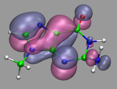
 In the next example a dissociation trajectory of an
Ar3+ molecule is shown. The color of the
VDW spheres shall indicate how the positive charge distributed
between the atoms with values ranging from 0.7 (coded blue) to 0.0
(coded red). Once more we load the trajectory (ar3plus.xyz and
ar3plus.dcd) in the regular way, visualize the Atoms as VDW
spheres, then read in the atom charges from
ar3plus-charge.dat, and store them in an
array. The procedure do_charge then updates the charge field
in of the atoms for the current frame. In contrast to the previous
example, the charge file is not stored per frame but for the
whole trajectory. So by tracing
vmd_frame($molid) we have this function being called
at every change of the animation frame number. The VMD code to
achieve this is as follows:
In the next example a dissociation trajectory of an
Ar3+ molecule is shown. The color of the
VDW spheres shall indicate how the positive charge distributed
between the atoms with values ranging from 0.7 (coded blue) to 0.0
(coded red). Once more we load the trajectory (ar3plus.xyz and
ar3plus.dcd) in the regular way, visualize the Atoms as VDW
spheres, then read in the atom charges from
ar3plus-charge.dat, and store them in an
array. The procedure do_charge then updates the charge field
in of the atoms for the current frame. In contrast to the previous
example, the charge file is not stored per frame but for the
whole trajectory. So by tracing
vmd_frame($molid) we have this function being called
at every change of the animation frame number. The VMD code to
achieve this is as follows:
set molid 0
# read in charge data
set n [molinfo $molid get numframes]
puts "reading charges"
set fp [open "ar3plus-charge.dat" r]
for {set i 0} {$i < $n} {incr i} {
    set chrg($i) [gets $fp]
}
close $fp

# procedure to change the charge field from the data in $chrg
proc do_charge {args} {
   global chrg molid
   set a [molinfo $molid get numatoms]
   set f [molinfo $molid get frame]
   for {set i 0} {$i < $a} {incr i} {
       set s [atomselect $molid "index $i"]
       $s set charge [lindex $chrg($f) $i]
   }
}

# turn on update of the charge info and coloring in each frame.
trace variable vmd_frame($molid) w do_charge
mol colupdate   0 $molid on

# set color mapping parameters
mol scaleminmax 0 $molid 0.0 0.7
color scale method RGB
color scale midpoint 0.25
color scale min 0.0
color scale max 0.7
# go back to the beginning and activate the additional feartures.
animate goto start
do_charge
|
The complete script of this visualization is also available for download under the name ar3plus-charge.vmd.
Full Table of Contents
![]()
1. Introduction
1.1. About this Tutorial
1.2. About the Programs
1.3. Notes
1.4. Citation / Bookmark
1.5. Recent Changes
2. Table of Contents
3. Preparation and Installation Issues
3.1. Customizing the VMD Setup
3.2. Predefining Additional Items
3.3. Extending the Script and Plugin Search Path
4. Loading and Displaying Configurations and Trajectories
4.1. Loading a Single Geometry
4.2. Creating a Visualization
4.3. Saving and Re-using a Visualization
4.4. Viewing a Trajectory
4.5. How to Show Breaking and Formation of Bonds
4.6. Adding Graphics to a Visualization
5. Adding Dynamic Graphics to a Trajectory
5.1. Adding a Progress Bar for the Elapsed Time
5.2. Display the Total Dipole Moment of the Simulation Cell
5.3. Visualizing Changing Atom Properties with Color
5.4. Modify an Atom Property Dynamically from an External File
6. Dynamic Atom Selection
6.1. Display a Changing Number of Molecules
6.2. Keeping Atoms or a Molecule in the Center and Aligned
6.3. Modify a Selection During a Trajectory
6.4. Using the User Field for Computed Selections
6.5. Tracing a Dynamic Property
7. Visualizing Volumetric Data from Cube-Files
7.1. Electron Density and Electrostatic Potential
7.2. Canonical and Localized Orbitals
7.3. Electron Localization Function (ELF)
7.4. Manipulation of Cube Files / Response to an External Potential
7.5. Bulk Systems
7.6. Animations with Isosurfaces
7.7. Volumetric data from Gaussian
8. Using Data Processing to Tailor Data for VMD
8.1. Visualizing Path-Integral Trajectories
8.2. Extracting the Geometry Information from old CPMD Output Files
8.3. Removing Unneeded Parts From a Cube File
8.4. Extract Some Coordinates with Bounding Box Information
8.5. Creating 3d-Ramachandran Histograms
9. Misc Tips and Tricks
9.1. Collected 'draw' Extensions
9.2. Using a Different Default Visualization
9.3. Changing the Default vdW Radii
9.4. Reloading the Current Trajectory
9.5. Visualize a Trajectory With a Changing Number of Atoms or Bonds
9.6. Set the Unit Cell Information for a Whole Trajectory
9.7. Directly Print the Current Visualization
9.8. Transferring a Visualization from a Molecule to Others
9.9. Adding a TCL-Plugin to the Extensions Menu
9.10. Turn Off Output in Analysis Scripts
9.11. Automatically Turn on TCL mode in (X)Emacs for .vmd Files
10. Credits
11. Downloads
12. Script distribution policy
|
|
|
||
|
|||