|
|
|
|
Visualization and Analysis of Quantum Chemical and Molecular Dynamics Data with VMD Part 6 |
|
8. Using Data Processing to Tailor Data for VMD
![]()
8.1. Visualizing Path-Integral Trajectories
![]()
8.2. Extracting the Geometry Information from old CPMD Output Files
![]()
8.3. Removing Unneeded Parts From a Cube File
![]()
8.4. Extract Some Coordinates with Bounding Box Information
![]()
8.5. Creating 3d-Ramachandran Histograms
![]()
![]() Part 5
Part 5
![]() Part 7
Part 7
![]() Start
Start
![]() Contents
Contents
In some cases the existing data is not (well) suited to be read in for a VMD visualization, so it needs to be augmented or converted using external programs. Here are some examples.
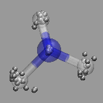
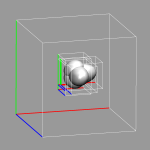
 In path integral simulations each atom is represented by several
replica, so reading in that data directly would create produce
several molecules positioned (almost) on top of each other, which
creates a somewhat cluttered visualization (see image on the right).
Therefore the atom positions are better taken as the average of the
replica and then a different, lucid visualization can be used.
The perl script
traj2xyz.pl will automatically detect path-integral runs
from the fact, that for technical reasons the GEOMETRY.xyz file
will only contain the geometry information for a single set of
replica atoms, and write out the average replica positions at the
beginning of each xyz record. The individual replica coordinates
can be recognized, since the script will prepend their name with
an X. Any selection with and not name "X.*" with ignore them.
The processed xyz file (nh3-pimd.xyz) and the visualization
(nh3-pimd.vmd) are available for download.
In path integral simulations each atom is represented by several
replica, so reading in that data directly would create produce
several molecules positioned (almost) on top of each other, which
creates a somewhat cluttered visualization (see image on the right).
Therefore the atom positions are better taken as the average of the
replica and then a different, lucid visualization can be used.
The perl script
traj2xyz.pl will automatically detect path-integral runs
from the fact, that for technical reasons the GEOMETRY.xyz file
will only contain the geometry information for a single set of
replica atoms, and write out the average replica positions at the
beginning of each xyz record. The individual replica coordinates
can be recognized, since the script will prepend their name with
an X. Any selection with and not name "X.*" with ignore them.
The processed xyz file (nh3-pimd.xyz) and the visualization
(nh3-pimd.vmd) are available for download.
When running geometry optimizations, having a look at the 'trajectory' of the optmization is often desirable. Newer CPMD versions support the XYZ flag to the OPTIMIZE GEOMETRY keyword to create an xyz-file that can be easily visualized, but for outputs from older CPMD versions (or in cases where setting the XYZ keyword was overlook or forgotten), one may want to extract the coordinates from the output file. Doing this with a text editor can be quite tiresome. The perl script out2xyz.pl will try to do this for you. Of course this script also works (or at least it should) for other jobs that contain geometry information.
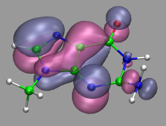
 Cubefiles can become quite large, especially for very large systems.
This can put a severy limit on how many of them can be visualized at
the same time or even stored on the same disk. Frequently only a part
of them is needed for the visualization, for example with surface slabs,
isolated molecules or when looking at localized orbitals. The trimcube
utility presented here (trimcube.c) allows to do this
almost automatically, by trying to cut off parts of a cube file, whose
absolute values are all below a given threshold. The version of
cpmd2cube distributed together CPMD v3.9.2 contains this feature
as well, so that you can get the small file immediately. The image on
the left shows the original box and then the subboxes for each localized
orbital. The file size reduction in this case was more than a factor of
35.
Cubefiles can become quite large, especially for very large systems.
This can put a severy limit on how many of them can be visualized at
the same time or even stored on the same disk. Frequently only a part
of them is needed for the visualization, for example with surface slabs,
isolated molecules or when looking at localized orbitals. The trimcube
utility presented here (trimcube.c) allows to do this
almost automatically, by trying to cut off parts of a cube file, whose
absolute values are all below a given threshold. The version of
cpmd2cube distributed together CPMD v3.9.2 contains this feature
as well, so that you can get the small file immediately. The image on
the left shows the original box and then the subboxes for each localized
orbital. The file size reduction in this case was more than a factor of
35.
trimcube: cut out a part of a cubefile. usage: trimcube [options] <input cube> [<output cube>] available options: -h[elp] print this info -t[hresh] <value> set trim threshold to <value>, (default 0.005) -n[orm] normalize so that the integral over the cube is zero. use '-' to read from standard input program writes to standard output if not output file is given |
To following script provides the command extract_sel (extract_sel.tcl) will write a pdb file from a given selection. The special feature is, that it will shift the selection close to the origin, compute a minimal box that will fit this selection and store it in the CRYST record of the pdb file. Very useful for creating a QM subsystem from a classical MD simulation.
proc extract_sel { sel pdbfile {addbox {2.0 2.0 2.0}} } {
  set molid [$sel molid]

  # save original box dimensions and selection coordinates
  set origbox [molinfo $molid get {a b c alpha beta gamma}]
  set origxyz [$sel get {x y z}]

  # get the min/max coordinates from the selection
  set minmax [measure minmax $sel]
  # subtract the coordinates of the lower left front corner.
  $sel moveby [vecscale -1.0 [lindex $minmax 0]]
  # and shift by half the addbox vector to the middle
  $sel moveby [vecscale 0.5 $addbox]

  # box shall be the size of the selection plus the addbox vector
  set box [vecsub [lindex $minmax 1] [lindex $minmax 0]]
  set box [vecadd $addbox $box]
  # update the box size so the pdbfile will get that info
  molinfo $molid set {a b c alpha beta gamma} "$box 90.0 90.0 90.0"
  $sel writepdb "$pdbfile"

  # undo the coordinate shifts from above and reset the box
  $sel set {x y z} $origxyz
  molinfo $molid set {a b c alpha beta gamma} $origbox
}
|
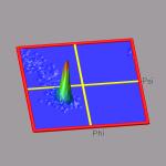
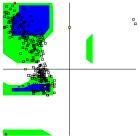 The ramaplot tool in VMD is very useful for tracking changes of the
protein backbone angles from a trajectory. But to get an impression of
the statistical distribution of some configurations, the 'show all
timesteps' mode in ramaplot can be easily misleading (see the picture on
the right). In this example we have a short trajectory of a 12-ALA alpha-helix
which is in fact stable during the time of the simulation.
A histogram of the data would put an equal weight to each data point and
with a so-called 'rubbersheet' representation (see picture on the left)
one could could identify the regions of statistical relevance much
better and see, that the alpha-helix does indeed not fall apart
significantly.
The ramaplot tool in VMD is very useful for tracking changes of the
protein backbone angles from a trajectory. But to get an impression of
the statistical distribution of some configurations, the 'show all
timesteps' mode in ramaplot can be easily misleading (see the picture on
the right). In this example we have a short trajectory of a 12-ALA alpha-helix
which is in fact stable during the time of the simulation.
A histogram of the data would put an equal weight to each data point and
with a so-called 'rubbersheet' representation (see picture on the left)
one could could identify the regions of statistical relevance much
better and see, that the alpha-helix does indeed not fall apart
significantly.
To achieve this, we have to first create a histogram of the alpha-carbon angles and then visualize it. Since VMD does not support this internally, we create an empty dummy molecule and add the surface to it using VMDs graphics primitives. With the following script code, we can create the raw histogram.
    set sel [atomselect top {protein and name CA}]
    set res 36
    set w [expr ($res - 1.0)/360.0]

    set n [molinfo [$sel molid] get numframes]
    for {set i 0 } { $i < $n } { incr i } {
        $sel frame $i
        $sel update

        foreach a [$sel get {phi psi}] {
            set phi [lindex $a 0]
            set psi [lindex $a 1]
            incr data([expr int(($phi + 180.0) * $w)],[expr int(($psi + 180.0) * $w)])
        }
    }
|
We then have to normalize the histogram and create the surface by drawing four triangles between the corners of each square of data points and their mid-point. We also use the z-value of the mid-point to colorize the triangles according to a BGR color scale. so that the bottom is blue and the peaks will be green with red tips:
    color scale method BGR
    color scale max 0.9
    color scale midpoint 0.3
    for {set i 0} {$i < $res} {incr i} {
        for {set j 0} {$j < $res} {incr j} {

            set i2 [expr $i + 1]
            set j2 [expr $j + 1]

            set x1 [expr ($i  - (0.5 * $res)) * $len]
            set x2 [expr ($i2 - (0.5 * $res)) * $len]
            set xm [expr 0.5 * ($x1 + $x2)]

            set y1 [expr ($j  - (0.5 * $res)) * $len]
            set y2 [expr ($j2 - (0.5 * $res)) * $len]
            set ym [expr 0.5 * ($y1 + $y2)]

            set zm [expr ($data($i,$j) + $data($i2,$j2) \
                        + $data($i2,$j) + $data($i,$j2)) / 4.0]

            graphics $mol color [expr 17 + int (200 * $zm)]

            graphics $mol triangle "$x1 $y1 $data($i,$j)"   \
                     "$xm $ym $zm" "$x2 $y1 $data($i2,$j)"
            graphics $mol triangle "$x1 $y1 $data($i,$j)" " \
                     $x1 $y2 $data($i,$j2)" "$xm $ym $zm"
            graphics $mol triangle "$x2 $y2 $data($i2,$j2)" \
                     "$x2 $y1 $data($i2,$j)" "$xm $ym $zm"
            graphics $mol triangle "$x2 $y2 $data($i2,$j2)" \
                     "$xm $ym $zm" "$x1 $y2 $data($i,$j2)"
        }
    }
|
Completed with a nice border and some labels the full code can be put into a separate subroutine, so that the code to create the picture on the left becomes:
mol new {12-ala.pdb} type pdb waitfor all
mol addfile {12-ala.dcd} type dcd waitfor all
set sel [atomselect top {resid > 1 and resid < 12 and name CA}]
mk3drama $sel
|
The VMD script code is available for download under
mk3drama.tcl. This subroutines also turns
off, but does not delete the originally loaded molecule(s),
so you can in fact create multiple histograms from different
selections and, e.g., view them in turn by clicking on
the 'D' symbols in the main VMD window. The visualization
and the data files are available under
12-ala-rama.vmd, 12-ala.pdb, and
12-ala.dcd.
Full Table of Contents
![]()
1. Introduction
1.1. About this Tutorial
1.2. About the Programs
1.3. Notes
1.4. Citation / Bookmark
1.5. Recent Changes
2. Table of Contents
3. Preparation and Installation Issues
3.1. Customizing the VMD Setup
3.2. Predefining Additional Items
3.3. Extending the Script and Plugin Search Path
4. Loading and Displaying Configurations and Trajectories
4.1. Loading a Single Geometry
4.2. Creating a Visualization
4.3. Saving and Re-using a Visualization
4.4. Viewing a Trajectory
4.5. How to Show Breaking and Formation of Bonds
4.6. Adding Graphics to a Visualization
5. Adding Dynamic Graphics to a Trajectory
5.1. Adding a Progress Bar for the Elapsed Time
5.2. Display the Total Dipole Moment of the Simulation Cell
5.3. Visualizing Changing Atom Properties with Color
5.4. Modify an Atom Property Dynamically from an External File
6. Dynamic Atom Selection
6.1. Display a Changing Number of Molecules
6.2. Keeping Atoms or a Molecule in the Center and Aligned
6.3. Modify a Selection During a Trajectory
6.4. Using the User Field for Computed Selections
6.5. Tracing a Dynamic Property
7. Visualizing Volumetric Data from Cube-Files
7.1. Electron Density and Electrostatic Potential
7.2. Canonical and Localized Orbitals
7.3. Electron Localization Function (ELF)
7.4. Manipulation of Cube Files / Response to an External Potential
7.5. Bulk Systems
7.6. Animations with Isosurfaces
7.7. Volumetric data from Gaussian
8. Using Data Processing to Tailor Data for VMD
8.1. Visualizing Path-Integral Trajectories
8.2. Extracting the Geometry Information from old CPMD Output Files
8.3. Removing Unneeded Parts From a Cube File
8.4. Extract Some Coordinates with Bounding Box Information
8.5. Creating 3d-Ramachandran Histograms
9. Misc Tips and Tricks
9.1. Collected 'draw' Extensions
9.2. Using a Different Default Visualization
9.3. Changing the Default vdW Radii
9.4. Reloading the Current Trajectory
9.5. Visualize a Trajectory With a Changing Number of Atoms or Bonds
9.6. Set the Unit Cell Information for a Whole Trajectory
9.7. Directly Print the Current Visualization
9.8. Transferring a Visualization from a Molecule to Others
9.9. Adding a TCL-Plugin to the Extensions Menu
9.10. Turn Off Output in Analysis Scripts
9.11. Automatically Turn on TCL mode in (X)Emacs for .vmd Files
10. Credits
11. Downloads
12. Script distribution policy
|
|
|
||
|
|||