|
|
|
|
Visualization and Analysis of Quantum Chemical and Molecular Dynamics Data with VMD Part 4 |
|
6. Dynamic Atom Selection
![]()
6.1. Display a Changing Number of Molecules
![]()
6.2. Keeping Atoms or a Molecule in the Center and Aligned
![]()
6.3. Modify a Selection During a Trajectory
![]()
6.4. Using the User Field for Computed Selections
![]()
6.5. Tracing a Dynamic Property
![]()
![]() Part 3
Part 3
![]() Part 5
Part 5
![]() Start
Start
![]() Contents
Contents
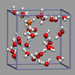
 Although this is not a problem unique to CPMD simulations,
here is one example on how you can program VMD to recalculate
the list of atoms or molecules fresh for each displayed timestep.
For the example shown on the left, a pair of solvent separated ions
(a sodium and a chloride) were selected from a (classical) molecular
dynamics simulation with 800 SPC/E waters 16 NaCl ion pairs. The ions
are represented by a VDW sphere and the first solvation shell waters
with a CPK style representation and 'regular' colors. The second
solvation shell ist transparent (cyan for the Na+ and lime
for the Cl-. Finally oxygens close to the interface between
the two solvation shells are highlighted in purple or in yellow. This
way you can more easily spot the exchange in the hydration shell of
the ions. As you can see from the animation, the chloride has larger
solvation shells with more exchange than the sodium and occasionally
water molecules in the second solvation shell are shared between both
ions.
Although this is not a problem unique to CPMD simulations,
here is one example on how you can program VMD to recalculate
the list of atoms or molecules fresh for each displayed timestep.
For the example shown on the left, a pair of solvent separated ions
(a sodium and a chloride) were selected from a (classical) molecular
dynamics simulation with 800 SPC/E waters 16 NaCl ion pairs. The ions
are represented by a VDW sphere and the first solvation shell waters
with a CPK style representation and 'regular' colors. The second
solvation shell ist transparent (cyan for the Na+ and lime
for the Cl-. Finally oxygens close to the interface between
the two solvation shells are highlighted in purple or in yellow. This
way you can more easily spot the exchange in the hydration shell of
the ions. As you can see from the animation, the chloride has larger
solvation shells with more exchange than the sodium and occasionally
water molecules in the second solvation shell are shared between both
ions.
Now how was this done? First we need to load the trajectory from the files 800h2o-16nacl.xyz and 800h2o-16nacl.dcd and delete the default representation. Next we define a set of atomselect macros that make the selection of the atoms much easier. Here is the block for the sodium hydration shells (the cutoff distances 3.3 and 5.5 were taken from the gNaO(r) function for this simulation).
# selection macros. this is the first part of the magic
atomselect macro hyd {name H}
atomselect macro oxy {name O}
# first and second solvation shell of Na+ and oxygens in transition
atomselect macro naox1 {oxy within 3.3 of index 2405}
atomselect macro naox2 {(oxy within 5.5 of index 2405) and not naox1}
atomselect macro naotr {(oxy within 3.35 of index 2405)
    and not (oxy within 3.25 of index 2405)}
atomselect macro nahy1 {hyd within 1.31 of naox1}
atomselect macro nahy2 {hyd within 1.31 of naox2}
|
Note how the hydrogens are selected with a distance criterium around the oxygen selections. This way you make sure that you select only complete water molecules for each shell. The selection for the chloride follows the same pattern.
The next step is to create the representations utilizing the selection macros. Finally you have to turn on recalculation of the selection for each representation (and we add a little trajectory smoothing to have a less jumpy animation). This is done with the following code:
# let all selections be recalculated for each frame
# and smooth the trajectory a little bit for all representations
# that's part two of the magic.
set molid 0
set n [molinfo $molid get numreps]
for {set i 0} {$i < $n} {incr i} {
    mol selupdate $i $molid on
    mol smoothrep $molid $i 2
}
# go back to the start of the trajectory.
animate goto start
|
That is it. How to display all hydrogen bonds for all visible water molecule is left to you as an exercise. The full VMD script file is also available for download under the name nacl-shell.vmd. There also is a somewhat larger (640x480 pixel, 4.7 MByte ) rendered MPEG-1 Movie of the same animation.
 There is some room for improvement in the previous example: the ion pair
rotates and moves around quite a bit (in fact it took considerable
amount of time to find an ion pair in the trajectory that stays
that much in place). For the solvated ion pair we want
to keep the ion pair centered and aligned along the x-axis. For that
we calculate the translation and rotation matrices with the trans
command by straightforward vector algebra. But using the center and
direction of the ion pair directly would give a very jumpy picture. So
we average both parameters over several frames (here 20) and used the
smoothed realignment instead. See the movie on the left as an example.
The code in nacl-follow.vmd differs from the previous
example primarily by the following, additional code:
There is some room for improvement in the previous example: the ion pair
rotates and moves around quite a bit (in fact it took considerable
amount of time to find an ion pair in the trajectory that stays
that much in place). For the solvated ion pair we want
to keep the ion pair centered and aligned along the x-axis. For that
we calculate the translation and rotation matrices with the trans
command by straightforward vector algebra. But using the center and
direction of the ion pair directly would give a very jumpy picture. So
we average both parameters over several frames (here 20) and used the
smoothed realignment instead. See the movie on the left as an example.
The code in nacl-follow.vmd differs from the previous
example primarily by the following, additional code:
proc do_realign {args} {
    global chist dhist hcount hoffs molid

    # this is the axis to align to
    set avec [vecnorm {1.0 0.0 0.0}]
    # this is the sliding window size
    set asize 20

    # initialize the cache counters
    if ([info exists hcount]) { } else {
        set hcount 0
        set hoffs  -1
    }

    # calculate center and direction of the ion pair
    set sel [atomselect $molid "index 2405 or index 2431"]
    lassign [$sel get {x y z}] na cl
    set cent [vecscale [vecadd $na $cl] 0.5]
    set dir [vecsub $na $cl]

    # store data in cache for sliding window averaring
    if {$hcount < $asize} then { incr hcount }
    incr hoffs
    if {$hoffs>= $hcount} then { set hoffs 0 }
    set chist($hoffs) $cent
    set dhist($hoffs) $dir

    # calculate averages
    set csum [veczero]
    set dsum [veczero]
    for {set i 0} {$i < $hcount} {incr i} {
        set csum [vecadd $csum $chist($i)]
        set dsum [vecadd $dsum $dhist($i)]
    }
    set csum [vecscale [expr 1.0/[expr $hcount * 1.0]] $csum]
    set dsum [vecnorm $dsum]

    # get rotation axis.
    set rvec [vecnorm [veccross $dsum $avec]]

    # set origin and rotation
    molinfo $molid set { center_matrix rotate_matrix} \
        [list [trans origin $csum] \
             [trans axis $rvec [expr acos([vecdot $dsum $avec])] rad]]
    # clean up selections
    $sel delete
}

trace variable vmd_frame($molid) w do_realign

# zoom to fit the display when vmd is started with '-size 800 600'
scale to 0.15
# the smoothing works better with this (no discontinuity)
animate style rock
|
 You will probably have noticed that running the previous two examples in VMD
needs somewhat more cpu power to get a smooth animation. This is because
all selections have to be recomputed anew in every animation step.
In cases where the selection mechanism is even more complicated
(and therefore more time consuming) you might want to find an
alternative way. Here are two suggestions: a) you compile lists of the
indices of the selected atoms with an external program, store
them in a file, read them into an array and replace the selection text
in each frame; b) you compute the selection directly, but then
cache the results in an array so that subsequent viewings of the same
frame are faster. In comparison, method a) has the advantage of being
faster even at the first viewing than b) but the drawback that you
have to keep and read in an additional (lengthy?) file.
You will probably have noticed that running the previous two examples in VMD
needs somewhat more cpu power to get a smooth animation. This is because
all selections have to be recomputed anew in every animation step.
In cases where the selection mechanism is even more complicated
(and therefore more time consuming) you might want to find an
alternative way. Here are two suggestions: a) you compile lists of the
indices of the selected atoms with an external program, store
them in a file, read them into an array and replace the selection text
in each frame; b) you compute the selection directly, but then
cache the results in an array so that subsequent viewings of the same
frame are faster. In comparison, method a) has the advantage of being
faster even at the first viewing than b) but the drawback that you
have to keep and read in an additional (lengthy?) file.
In the example on the left, oxygen(s) where the excess proton is within bonding radius (1.32 Angstrom, as taken from the radial pair distribution function) should get a yellow highlight. So we first create the representation, but set the selection to "none". Note the index for the selection; in our case it is 2.
For method a) we compute the selecting by index strings and write them to a file (h3oplus-select.dat). For viewing we read this file into an array and have the selection updated from this array. Here is the code to achieve this (h3oplus-select.vmd):
# function to update the selection from the highlight array
proc do_highlight {args} {
    global highlight molid selid
    # get the current frame number
    set frame [molinfo $molid get frame]
    # if we have data for this frame, update the selection
    if {[info exists highlight($frame)]} then {
        mol modselect $selid $molid "$highlight($frame)"
    }
}

set molid [molinfo top]
set selid 2
set n [molinfo $molid get numframes]
set highlight(0) none
# read selections from file
set fp [open "h3oplus-select.dat" r]
for {set i 0} {$i < $n} {incr i} {
    set highlight($i) [gets $fp]
}
close $fp

# hook highlight function into animation
trace variable vmd_frame($molid) w do_highlight
animate goto start
|
For method b) we put the code to compute the selection within the highlight function, but first check the array whether we have already computed the selection and then use the cached value instead. This example is available under the name h3oplus-cache.vmd:
# subroutine to update the selection of
# representation $selid and cache the results
proc do_highlight {args} {
    global highlight molid selid
    # get the current frame number
    set frame [molinfo $molid get frame]
    if {[info exists highlight($frame)]} then {
        mol modselect $selid $molid "$highlight($frame)"
    } else {
        set hl {none}
        # loop over all oxygens to count hydrogens within bondlength
        set osel [atomselect $molid "name O"]
        foreach ox [$osel list] {
            set sel [atomselect $molid "name H and within 1.32 of index $ox"]
            $sel frame $frame
            $sel update
            if {[$sel num] != 2 } {
                set hl "$hl or index $ox"
            }
            $sel delete
        }
        $osel delete
        # apply new selection and cache it
        mol modselect $selid $molid "$hl"
        set highlight($frame) "$hl"
    }
}

set molid [molinfo top]
set selid 2

trace variable vmd_frame($molid) w do_highlight
animate goto start
|
With recent versions of VMD the user field allows to store properties for each frame for each atom and which can be accessed in selection expressions. Using this method on the previous example one would first need to compute the number of bonded Hydrogens and store it in the user field. Using selections for that avoids the time consuming computations in Tcl and thus combines the advantages of both methods presented above.
# prep
set num [molinfo $mol get numframes]
set ox  [atomselect $mol {name O}]
set all [atomselect $mol {all}]

# create a selection for each oxygen atom to compute
foreach i [$ox get index] {
    set sel($i) [atomselect $mol "exwithin 1.30 of index $i"]
}

# loop over all frames, and for each frame loop over
# all oxygens and store the number of hydrogens in user
for {set n 0} {$n < $num} {incr n} {
    set bc {}
    foreach i [$ox get index] {
        $sel($i) frame $n
        $sel($i) update
        $all frame $n
        $all set user 0
        lappend bc [$sel($i) num]
    }
    $ox frame $n
    $ox set user $bc
    unset bc
}

# clean up selections
foreach i [$ox get index] {
    $sel($i) delete
}
$ox delete
$all delete
unset ox all sel i n
|
Now to recognize all Oxygen atoms with more than two bonded Hydrogens, we simply need to define a selection with user > 2 and make sure that the selection is evaluated for every frame during an animation (-> Trajectory tab in the Graphical Representations menu.
mol representation VDW 0.60000 20.000000
mol color ColorID 4
mol selection {name O and user > 2}
mol material Transparent
mol addrep top
mol selupdate 3 $mol on
|
The complete example is available for download: 32h2o_h3op_user.vmd.
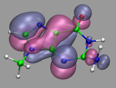
Sometimes you want to show the dynamics of a process but are not able to use an animation. The trajectory_path procedure from the VMD script library is a nice example for that and can be used for the proton transport example from above as well, after it was adapted to allow updating the selection during the tracing of the path. Compared to the original, trajectory_path.tcl, has two additional, optional arguments to turn on/off the selection update and set the linewidth. The image on the left was created with the VMD script from above plus the following additional code (32h2o_h3op_trace.vmd).
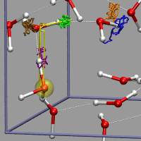
# create selection for tracing hydrogens and the h3o-plus
set hyd1 [atomselect $mol {index 85}]
set hyd2 [atomselect $mol {index 99}]
set hyd3 [atomselect $mol {index 86}]
set hyd4 [atomselect $mol {index 97}]
set hyd5 [atomselect $mol {index 98}]
set h3op [atomselect $mol {name O and user > 2}]

# draw trajectory paths
trajectory_path $hyd1 blue 0 4
trajectory_path $hyd2 green 0 4
trajectory_path $hyd3 orange 0 4
trajectory_path $hyd4 purple 0 4
trajectory_path $hyd5 ochre 0 4
trajectory_path $h3op yellow 1 4
|
The image demonstrates nicely and without any animation, that the excess proton 'defect' is much more movable than the individual Hydrogen atoms due to the Grotthuss structural diffusion mechanism.
Full Table of Contents
![]()
1. Introduction
1.1. About this Tutorial
1.2. About the Programs
1.3. Notes
1.4. Citation / Bookmark
1.5. Recent Changes
2. Table of Contents
3. Preparation and Installation Issues
3.1. Customizing the VMD Setup
3.2. Predefining Additional Items
3.3. Extending the Script and Plugin Search Path
4. Loading and Displaying Configurations and Trajectories
4.1. Loading a Single Geometry
4.2. Creating a Visualization
4.3. Saving and Re-using a Visualization
4.4. Viewing a Trajectory
4.5. How to Show Breaking and Formation of Bonds
4.6. Adding Graphics to a Visualization
5. Adding Dynamic Graphics to a Trajectory
5.1. Adding a Progress Bar for the Elapsed Time
5.2. Display the Total Dipole Moment of the Simulation Cell
5.3. Visualizing Changing Atom Properties with Color
5.4. Modify an Atom Property Dynamically from an External File
6. Dynamic Atom Selection
6.1. Display a Changing Number of Molecules
6.2. Keeping Atoms or a Molecule in the Center and Aligned
6.3. Modify a Selection During a Trajectory
6.4. Using the User Field for Computed Selections
6.5. Tracing a Dynamic Property
7. Visualizing Volumetric Data from Cube-Files
7.1. Electron Density and Electrostatic Potential
7.2. Canonical and Localized Orbitals
7.3. Electron Localization Function (ELF)
7.4. Manipulation of Cube Files / Response to an External Potential
7.5. Bulk Systems
7.6. Animations with Isosurfaces
7.7. Volumetric data from Gaussian
8. Using Data Processing to Tailor Data for VMD
8.1. Visualizing Path-Integral Trajectories
8.2. Extracting the Geometry Information from old CPMD Output Files
8.3. Removing Unneeded Parts From a Cube File
8.4. Extract Some Coordinates with Bounding Box Information
8.5. Creating 3d-Ramachandran Histograms
9. Misc Tips and Tricks
9.1. Collected 'draw' Extensions
9.2. Using a Different Default Visualization
9.3. Changing the Default vdW Radii
9.4. Reloading the Current Trajectory
9.5. Visualize a Trajectory With a Changing Number of Atoms or Bonds
9.6. Set the Unit Cell Information for a Whole Trajectory
9.7. Directly Print the Current Visualization
9.8. Transferring a Visualization from a Molecule to Others
9.9. Adding a TCL-Plugin to the Extensions Menu
9.10. Turn Off Output in Analysis Scripts
9.11. Automatically Turn on TCL mode in (X)Emacs for .vmd Files
10. Credits
11. Downloads
12. Script distribution policy
|
|
|
||
|
|||