CPMD Tutorial

Theoretische Chemie, Ruhr-Universität Bochum,Germany http://www.theochem.ruhr-uni-bochum.de/go/cpmd-tutor.html

CPMD Tutorial

Part 3

    5. The Basics: Running CPMD, Input and Output Formats

         5.1. Wavefunction Optimization: a) Input File Format

         5.2. Wavefunction Optimization: b) Output File Format

    Part 2     Part 4     Start     Contents

5. The Basics: Running CPMD, Input and Output Formats

Electron redistribution of Hydrogen The first example will demonstrate some of the basic steps of performing a CPMD calculation with a very simple molecule: hydrogen, and a very simple task: calculate the electronic structure. We will use that as an example to have a look at the input file format, and how to read the output.

5.1. Wavefunction Optimization: a) Input File Format

For nearly all CPMD calculations, you first have to calculate the electron structure of your system, and use that as a base for further calculations. For our first calculation you'll need the input file 1-h2-wave.inp and the pseudo-potential file H_MT_LDA.psp

Now let's have a look at the input file. The input is organized in sections which start with &NAME and end with &END. Everything outside those sections is ignored. Also all keywords have to be in upper case or else they will be ignored. The sequence of the sections does not matter, nor does the order of keywords, except where noted in the manual. A minimal input file must have a &CPMD, &SYSTEM and an &ATOMS section. For more details on the input syntax, please have a look at the CPMD manual.

&INFO isolated hydrogen molecule. single point calculation. &END

The input file starts with an (optional) &INFO section. This section allows you to put comments about the calculation into the input file and they will be repeated in the output file. This can be very useful to match input and output files.

&CPMD OPTIMIZE WAVEFUNCTION CONVERGENCE ORBITALS 1.0d-7

This first part of &CPMD section instructs the program to do a wavefunction optimization (i.e. a single point calculation) with a very tight convergence criterion (the default is 1.0d-5).

CENTER MOLECULE ON PRINT FORCES ON &END

The rest of the &CPMD section has the molecule moved to the center of the simulation cell and asks to calculate and print the forces on each atom at the end of the run.

&SYSTEM SYMMETRY 1 ANGSTROM CELL 8.00 1.0 1.0 0.0 0.0 0.0 CUTOFF 70.0 &END

The &SYSTEM section contains various parameters related to the simulations cell and the representation of the electronic structure. The keywords SYMMETRY, CELL and CUTOFF are required and define the (periodic) symmetry, shape, and size of the simulation cell, as well as the plane wave cutoff (i.e. the size of the basis set). The keyword ANGSTROM additionally indicates that all lengths and coordinates are given in angstrom (and not in a.u.).

&DFT FUNCTIONAL LDA &END

The &DFT section is used to select the density functional and related parameters. In this case we go with the local density approximation (which also is the default).

&ATOMS *H_MT_LDA.psp LMAX=S 2 4.371 4.000 4.000 3.629 4.000 4.000 &END

Finally the &ATOMS section is needed to specify the atom coordinates and the pseudopotentials, that are used to represent them. The detailed syntax of the pseudopotential specification is a bit complicated and will not be needed nor discussed here. If you want to know more, please have a look at the Further Details of the Input section of the CPMD manual.

5.2. Wavefunction Optimization: b) Output File Format

Now type:

cpmd.x 1-h2-wave.inp> 1-h2-wave.out

to start the calculation, which should be completed in less than a minute. The main output of the CPMD program is now in the file 1-h2-wave.out. Let's have a closer look at the contents of this file.

PROGRAM CPMD STARTED AT: Tue Nov 9 15:47:26 2004 ****** ****** **** **** ****** ******* ******* ********** ******* *** ** *** ** **** ** ** *** ** ** *** ** ** ** ** ** ** ******* ** ** ** ** *** ****** ** ** ** *** ******* ** ** ** ******* ****** ** ** ** ****** VERSION 3.9.1 COPYRIGHT IBM RESEARCH DIVISION MPI FESTKOERPERFORSCHUNG STUTTGART The CPMD consortium WWW: http://www.cpmd.org Mailinglist: cpmd-list@cpmd.org E-mail: cpmd@cpmd.org *** Nov 7 2004 -- 20:54:03 ***

We start with the header, where you can see, when the run was started, what version on CPMD you were using, and when it was compiled.

THE INPUT FILE IS: h2-wave.inp THIS JOB RUNS ON: yello.theochem.ruhr-uni-bochum.de THE CURRENT DIRECTORY IS: /rubberbandman/akohlmey/Barcelona_axel/devel/handout THE TEMPORARY DIRECTORY IS: /rubberbandman/akohlmey/Barcelona_axel/devel/handout THE PROCESS ID IS: 14621

Here we have some technical information about the environment, where this job was run.

****************************************************************************** * INFO - INFO - INFO - INFO - INFO - INFO - INFO - INFO - INFO - INFO - INFO * ****************************************************************************** * isolated hydrogen molecule. * * single point calculation. * ******************************************************************************

Here we see the contents of the &INFO section copied to the output.

SINGLE POINT DENSITY OPTIMIZATION PATH TO THE RESTART FILES: ./ GRAM-SCHMIDT ORTHOGONALIZATION MAXIMUM NUMBER OF STEPS: 10000 STEPS PRINT INTERMEDIATE RESULTS EVERY 10001 STEPS STORE INTERMEDIATE RESULTS EVERY 10001 STEPS NUMBER OF DISTINCT RESTART FILES: 1 TEMPERATURE IS CALCULATED ASSUMING EXTENDED BULK BEHAVIOR FICTITIOUS ELECTRON MASS: 400.0000 TIME STEP FOR ELECTRONS: 5.0000 TIME STEP FOR IONS: 5.0000 CONVERGENCE CRITERIA FOR WAVEFUNCTION OPTIMIZATION: 1.0000E-07 WAVEFUNCTION OPTIMIZATION BY PRECONDITIONED DIIS THRESHOLD FOR THE WF-HESSIAN IS 0.5000 MAXIMUM NUMBER OF VECTORS RETAINED FOR DIIS: 10 STEPS UNTIL DIIS RESET ON POOR PROGRESS: 10 FULL ELECTRONIC GRADIENT IS USED SPLINE INTERPOLATION IN G-SPACE FOR PSEUDOPOTENTIAL FUNCTIONS NUMBER OF SPLINE POINTS: 5000

This section now gives you a summary of the parameters read in from the &CPMD section, or their respective default settings.

EXCHANGE CORRELATION FUNCTIONALS LDA EXCHANGE: NONE LDA XC THROUGH PADE APPROXIMATION S.GOEDECKER, J.HUTTER, M.TETER PRB 54 1703 (1996) *** DETSP| THE NEW SIZE OF THE PROGRAM IS 1528/ 43068 kBYTES *** ***************************** ATOMS **************************** NR TYPE X(bohr) Y(bohr) Z(bohr) MBL 1 H 8.259992 7.558904 7.558904 3 2 H 6.857816 7.558904 7.558904 3 **************************************************************** NUMBER OF STATES: 1 NUMBER OF ELECTRONS: 2.00000 CHARGE: 0.00000 ELECTRON TEMPERATURE(KELVIN): 0.00000 OCCUPATION 2.0 [...] **************************************************************** * ATOM MASS RAGGIO NLCC PSEUDOPOTENTIAL * * H 1.0080 1.2000 NO S LOCAL * ****************************************************************

This part of the output tells you which and how many atoms and electrons are used, what functional and what pseudopotentials were used, and what the values of some related parameters are.

************************** SUPERCELL *************************** SYMMETRY: SIMPLE CUBIC LATTICE CONSTANT(a.u.): 15.11781 CELL DIMENSION: 15.1178 1.0000 1.0000 0.0000 0.0000 0.0000 VOLUME(OMEGA IN BOHR^3): 3455.14651 LATTICE VECTOR A1(BOHR): 15.1178 0.0000 0.0000 LATTICE VECTOR A2(BOHR): 0.0000 15.1178 0.0000 LATTICE VECTOR A3(BOHR): 0.0000 0.0000 15.1178 RECIP. LAT. VEC. B1(2Pi/BOHR): 0.0661 0.0000 0.0000 RECIP. LAT. VEC. B2(2Pi/BOHR): 0.0000 0.0661 0.0000 RECIP. LAT. VEC. B3(2Pi/BOHR): 0.0000 0.0000 0.0661 REAL SPACE MESH: 90 90 90 WAVEFUNCTION CUTOFF(RYDBERG): 70.00000 DENSITY CUTOFF(RYDBERG): (DUAL= 4.00) 280.00000 NUMBER OF PLANE WAVES FOR WAVEFUNCTION CUTOFF: 17133 NUMBER OF PLANE WAVES FOR DENSITY CUTOFF: 136605 ****************************************************************

This part of the output presents the settings read in from the &SYSTEM section of the input file and some derived parameters.

[...] (K+E1+L+N+X) TOTAL ENERGY = -1.09689769 A.U. (K) KINETIC ENERGY = 0.81247073 A.U. (E1=A-S+R) ELECTROSTATIC ENERGY = -0.48640049 A.U. (S) ESELF = 0.66490380 A.U. (R) ESR = 0.17302596 A.U. (L) LOCAL PSEUDOPOTENTIAL ENERGY = -0.84879443 A.U. (N) N-L PSEUDOPOTENTIAL ENERGY = 0.00000000 A.U. (X) EXCHANGE-CORRELATION ENERGY = -0.57417350 A.U.

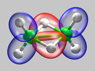
After some output to report the setup of the initial guess for the electron structure, we now see a summary of the various energy contribution of to the total energy of the system, based on the initial guess. Now the program is ready to start the wavefunction optimization. The image illustrates, how the electron density is redistributed: density from the blue area is moved to the red area.

Starting from the initial guess based on atomic wavefunctions the wavefunction for the total system is now calculated with an optimization procedure. You can follow the progress of the optimization in the output file.

NFI GEMAX CNORM ETOT DETOT TCPU 1 3.816E-02 2.886E-03 -1.096898 0.000E+00 1.61 2 8.628E-03 1.041E-03 -1.130803 -3.391E-02 1.64 3 2.736E-03 2.293E-04 -1.132376 -1.572E-03 1.63 4 6.115E-04 4.235E-05 -1.132456 -8.056E-05 1.65 5 1.532E-04 7.007E-06 -1.132459 -3.315E-06 1.66 6 3.895E-05 1.396E-06 -1.132460 -1.338E-07 1.65 7 6.271E-06 4.451E-07 -1.132460 -7.716E-09 1.64 8 7.764E-07 1.274E-07 -1.132460 -4.268E-10 1.69 9 1.317E-07 2.819E-08 -1.132460 -1.993E-11 1.65 10 1.871E-08 5.247E-09 -1.132460 -8.300E-13 1.67

Electron redistribution in Hydrogen during WF-optimization

The columns have the following meaning:
NFI:	Step number (number of finite iterations)
GEMAX:	largest off-diagonal component
CNORM:	average of the off-diagonal components
ETOT:	total energy
DETOT:	change in total energy to the previous step
TCPU:	(CPU) time for this step.

And you can see that the calculation stops after the convergence criterion of 1.0d-7 has been reached for the GEMAX value.

**************************************************************** * * * FINAL RESULTS * * * **************************************************************** ATOM COORDINATES GRADIENTS (-FORCES) 1 H 8.2600 7.5589 7.5589 1.780E-02 -1.327E-16 -9.739E-17 2 H 6.8578 7.5589 7.5589 -1.780E-02 -2.065E-16 -1.807E-16 **************************************************************** ELECTRONIC GRADIENT: MAX. COMPONENT = 9.23124E-09 NORM = 1.05089E-09 NUCLEAR GRADIENT: MAX. COMPONENT = 1.77986E-02 NORM = 1.02760E-02 TOTAL INTEGRATED ELECTRONIC DENSITY IN G-SPACE = 2.000000 IN R-SPACE = 2.000000 (K+E1+L+N+X) TOTAL ENERGY = -1.13245953 A.U. (K) KINETIC ENERGY = 1.09007154 A.U. (E1=A-S+R) ELECTROSTATIC ENERGY = -0.47319172 A.U. (S) ESELF = 0.66490380 A.U. (R) ESR = 0.17302596 A.U. (L) LOCAL PSEUDOPOTENTIAL ENERGY = -1.09902235 A.U. (N) N-L PSEUDOPOTENTIAL ENERGY = 0.00000000 A.U. (X) EXCHANGE-CORRELATION ENERGY = -0.65031700 A.U. ****************************************************************

Here we have the final summary of the results from our single point calculation. Since we have requested the output of the (atomic) forces you can see them alongside the atom coordinates. Please note, that regardless of the input units, coordinates in the CPMD output are always in atomic units. Although the calculation started with the experimental H-H bond length there are still some significant forces in the direction of the molecular axis. A clear indication, that within the approximations used in this calculation the equilibrium H-H distance lies somewhere else (but not too far away).

================================================================ BIG MEMORY ALLOCATIONS XF 1507142 PSI 1507142 YF 1507142 SCR 1026981 RHOE 753571 GK 409815 SCG 273210 INYH 204908 PME 171410 RHOPS 136605 ---------------------------------------------------------------- [PEAK NUMBER 78] PEAK MEMORY 8512086 = 68.1 MBytes ================================================================ **************************************************************** * * * TIMING * * * **************************************************************** SUBROUTINE CALLS CPU TIME ELAPSED TIME S_INVFFT 26 2.82 2.84 INVFFT 14 2.77 2.76 FWFFT 13 2.56 2.58 FFT-G/S 80 2.50 2.53 XCENER 13 2.19 2.22 VOFRHOB 13 1.66 1.69 S_FWFFT 14 1.64 1.64 RHOOFR 12 1.53 1.56 VPSI 14 1.51 1.54 ATRHO 1 1.14 1.19 VOFRHOA 13 0.99 0.97 PHASE 27 0.89 0.89 EICALC 13 0.67 0.70 ODIIS 12 0.49 0.49 RGGEN 1 0.22 0.22 FORMFN 1 0.21 0.21 NUMPW 1 0.13 0.13 RGS 12 0.03 0.04 PUTPS 1 0.03 0.03 ---------------------------------------------------------------- TOTAL TIME 23.98 24.21 **************************************************************** CPU TIME : 0 HOURS 0 MINUTES 24.11 SECONDS ELAPSED TIME : 0 HOURS 0 MINUTES 24.45 SECONDS PROGRAM CPMD ENDED AT: Tue Nov 9 15:47:48 2004

In the final part of the output, we see some statistics regarding memory and CPU time usage. This is mainly of interest for CPMD developers, but it does not hurt to have an occasional look and see if the numbers are reasonable. Please note, that the retrieval of this information is highly platform dependent, and that on some platforms the output may be bogus or very unreliable.

Other Output Files:

Apart from the console output, our CPMD run created a few other files. Most importantly the restart file RESTART.1 and its companion file LATEST. The restart file contains the final state of the system when the program terminated. This is needed to start other calculations, which need a converged wavefunction as a starting point. The file GEOMETRY.xyz contains the coordinates of the atoms in a format, that can be read in by many molecular visualization programs. The other files (e.g. GSHELL, GEOMETRY) can be ignored.

Top of Page

Part 2

Part 4

Start

PDF version of this document.

Full Table of Contents

1. Introduction
     1.1. Development Notice
     1.2. Notes
     1.3. Recent Changes
     1.4. Citation / Bookmark
2. Table of Contents
3. Preparation and Installation Issues
     3.1. Compiling CPMD
     3.2. Running CPMD
     3.3. Running cpmd2cube
4. The Theory: Some Fundamental Infos and Useful Literature
5. The Basics: Running CPMD, Input and Output Formats
     5.1. Wavefunction Optimization: a) Input File Format
     5.2. Wavefunction Optimization: b) Output File Format
     5.3. Geometry Optimization
     5.4. Car-Parrinello Molecular Dynamics
     5.5. Further Job Types
     5.6. How to Use the Tutorial
6. Exercise: Electron Structure and Geometry Optimization
     6.1. Hydrogen Molecule
     6.2. Water Molecule
     6.3. Ammonia Molecule
7. Exercise: Car-Parrinello Molecular Dynamics
     7.1. Hydrogen Molecule
     7.2. Ammonia Molecule in Gas Phase
     7.3. Glycine Molecule in Gas Phase
     7.4. Glycine with Thermostats
8. Exercise: Bulk Systems
     8.1. Bulk Silicon
     8.2. Hydronium Ion in Bulk Water
9. Exercise: Determination of Dynamic Properties
     9.1. Calculation of Vibrational Spectra
     9.2. The 'Dragging Effect'
10. Proton Transfer in a Catalytic Triade Model
     10.1. Preparing a Model from a Large System
     10.2. Equilibration with a Blocked Reaction Path
     10.3. Modelling Part of the Reaction Path
     10.4. Calculating Electron Structure Properties and Visualizations
11. Credits
12. Downloads
13. File distribution policy

Theoretische Chemie, Ruhr-Universität Bochum,Germany http://www.theochem.ruhr-uni-bochum.de/go/cpmd-tutor.html

Homepage Axel Kohlmeyer

Disclaimer / E-mail to the webmaster of this hompage: webmaster@theochem.ruhr-uni-bochum.de
Source File: index.wml (Sat Jul 2 18:07:27 2005) ($Revision: 1.16 $) Translated to HTML: Mon Oct 10 00:06:26 2005