|
|
|
|
CPMD Tutorial Part 6 |
|
7. Exercise: Car-Parrinello Molecular Dynamics
![]()
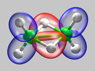
7.1. Hydrogen Molecule
![]()
7.2. Ammonia Molecule in Gas Phase
![]()
7.3. Glycine Molecule in Gas Phase
![]()
7.4. Glycine with Thermostats
![]()
![]() Part 5
Part 5
![]() Part 7
Part 7
![]() Start
Start
![]() Contents
Contents
 For our first real Car-Parrinello MD simulations we
start again small and simple: with the hydrogen molecule.
For the following MD calculations you can re-use the RESTART
file
from the previous calculations
or create a new one from the file
1-h2-wave.inp.
For our first real Car-Parrinello MD simulations we
start again small and simple: with the hydrogen molecule.
For the following MD calculations you can re-use the RESTART
file
from the previous calculations
or create a new one from the file
1-h2-wave.inp.
From the previously optimized electron structure, we start some MD calculations for different timesteps (6a-h2-md-5au.inp, 6b-h2-md-4au.inp, 6c-h2-md-3au.inp). Since the pre-optimized wavefunction is done for an optimized geometry, we have to add some kinetic energy to the system to 'see some action'. This is done via the keyword:
TEMPERATURE 50.0d0 |
Note that TEMPERATURE does not 'control' the temperature in any way, but only sets the initial kinetic energy of the system. Since we started from an optimized geometry, the average temperature during the simulation will be significantly lower.
Please save the files ENERGIES and TRAJEC.xyz from each of those runs and compare them later using the appropriate visualization programs. What is the effect of the different time steps?
ANNEALING ELECTRONS 0.98 |
Requirements: Memory: 50-100 MB, CPU time: 30-45 min.
As a next example we start an MD with ultra-soft pseudopotentials, starting from the restart of the optimized pyramidal (1-nh3-geoopt-vdb.inp) configuration.
First we try to bring the system (roughly) into an equilibrium at 700K. This is most efficiently done by initializing the kinetic energy and then rescaling the velocities of the atoms whenever the instantaneous temperature is more than 50 Kelvin away from the target temperature of 700K. This is done by using (5-nh3-md-vdb.inp):
TEMPERATURE 700.0 TEMPCONTROL IONS 700.0 50.0 |
Now we want to continue without thermostatting, so those four lines are removed. But we want to continue the trajectory uninterrupted, so we have to read the in the velocities (for the electronic degrees of freedom as well as for the atoms). We do not rename the RESTART.1 file, but have CPMD directly restart from the last restart via the LATEST keyword. But you should rename the TRAJEC.xyz and the ENERGIES file, so that we have seperate files for both parts of the trajectory (if you don't they will get appended, so you would have to cut them in parts later). When visualizing the trajectory, you may have notice, that the molecule translates and rotates. This is not ideal for an isolated molecule, but due to the intial starting conditions and numerical errors, those (unphysical) translational and rotational movement will always be there, and through the temperature control with rescaling they usually get emphasized as well. Since we want to look at an isolated molecule, we therefore redistribute the energy from those degrees of freedom to the rest by using the keyword SUBTRACT. Alltogether after removing the lines from above, we have to add the following lines (6-nh3-md-cont.inp):
RESTART WAVEFUNCTION COORDINATES VELOCITIES LATEST SUBTRACT COMVEL ROTVEL 25 |
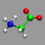 By now we should be ready to create a first CPMD input file (almost)
from scratch. We want to do an CP-MD simulation of an isolated glycine
molecule. You can use the coordinates from the file
gly.xyz and use the Ammonia
molecule input as a template. Check out the CPMD manual for the supercell
size requirements for the TUCKERMAN Poisson solver.
By now we should be ready to create a first CPMD input file (almost)
from scratch. We want to do an CP-MD simulation of an isolated glycine
molecule. You can use the coordinates from the file
gly.xyz and use the Ammonia
molecule input as a template. Check out the CPMD manual for the supercell
size requirements for the TUCKERMAN Poisson solver.
Best you start with a wavefunction optimization with a very tiny cutoff (5 ry) and MAXSTEP set to 1. This is the fastest way to debug your input file (the wavefunction of that run is useless). Also compare the resulting GEOMETRY.xyz file with the example coordinates and see if the geometry is read correctly. Keep in mind, that SYMMETRY 0 implies centering of the molecule in the supercell.
Now modify the &CPMD and &SYSTEM sections of your input file to be able to do a geometry optimization, using the proper plane wave cutoff. This is usually a good idea if you don't have an equilibrium geometry to start from or are using coordinates from a molecule editor program. This way you make sure, that you don't have too much potential energy in your system and it won't 'explode'.
Now start a CP-MD simulation using the wavefunction and coordinates from the previous calculation and equilibrate the molecule for 500 steps to 300K via velocity rescaling. Please rename the ENERGIES, TRAJECTORY, TRAJEC.xyz files so that the following run does not append to them.
Now turn off the velocity rescaling to continue with a production run without any temperature control (microcanonical ensemble) for (at least) 2000 steps. Note that you now have to read the velocities from the restart as well. Also you should only record every 10th step of the trajectory (using TRAJECTORY SAMPLE), so you don't get a too large file (the time step is rather small so you would not see much difference between the individual configurations anyways). Finally you should add
RESTFILE 4 STORE 500 |
to the &CPMD section which will write a restart file every 500 steps and name them alternating RESTART.1, RESTART.2, RESTART.3, and RESTART.4. Thus you won't lose too much of your calculation if the job gets terminated for some reason in the middle of the trajectory. Using multiple restarts provides extra security in case there is file system corruption or the simulation starts behaving erratically at some point. CPMD simulations usually need a lot of computational effort, so it is good practice to avoid having to redo too much of a simulation in any case.
Monitor the various energies during the run. How do they correspond to the movement of the atoms?
Requirements: Memory: 100 MB, CPU time: 10+30 min, equilibration, >6h h production.
For longer production MD simulations one usually couples the system to a heat bath via a thermostat algorithm. This is primarily done to compensate for small drift in the total energy due to numerical inaccuracies that accumulate slowly over the course of the simulation. Also the canonical NVT ensemble is usually more suited for calculation of thermodynamic properties than the microcanonical NVE ensemble.
For a simulation of a molecule in the gas phase the use of the MASSIVE thermostat is strongly recommended. In this context, massive does not refer to a more 'strict' or 'powerful' thermostat, but to a separate thermostat chain for each degree of freedom, i.e. massive referes to the total number of thermostats. This way a proper sampling of phase space is ensured, even if the various vibrational modes of the molecule(s) are only weakly coupled to the heat bath.
The thermostat for the electrons should be adjusted so that the target 'temperature' should be roughly the average value of EKINC in the later part of previous uncontrolled simulation. Good values for the characteristic frequency of the electrons and ions here are 10000.0 to 15000.0 and 2500.0 to 4000.0, respectively.
If you want to restart with active Nose thermostats, you need to read the state of the thermostat from the restart as well with adding NOSEE and NOSEP to the RESTART keyword for the electron and ion thermostats. If you change the thermostat algorithm (i.e. turn it on or off) you should not use those keywords and use RESCALE OLD VELOCITIES instead.
Based on the information presented in the section (and additional help from the CPMD manual if needed) we want to continue the previously uncontrolled CP-MD simulation of the glycine molecule with Nose thermostats for the electrons and atoms (at 300K). If the microcanonical CP-MD run from the previous run is not yet finished, you can initiate a graceful exit (i.e. one the produces a restart file) by creating a file named EXIT in the working directory of the CPMD run (e.g. by typing 'touch EXIT' , ': > EXIT' , or 'echo > EXIT' ).
Requirements: Memory: 250 MB, CPU time: up to a few days..
Full Table of Contents
![]()
1. Introduction
1.1. Development Notice
1.2. Notes
1.3. Recent Changes
1.4. Citation / Bookmark
2. Table of Contents
3. Preparation and Installation Issues
3.1. Compiling CPMD
3.2. Running CPMD
3.3. Running cpmd2cube
4. The Theory: Some Fundamental Infos and Useful Literature
5. The Basics: Running CPMD, Input and Output Formats
5.1. Wavefunction Optimization: a) Input File Format
5.2. Wavefunction Optimization: b) Output File Format
5.3. Geometry Optimization
5.4. Car-Parrinello Molecular Dynamics
5.5. Further Job Types
5.6. How to Use the Tutorial
6. Exercise: Electron Structure and Geometry Optimization
6.1. Hydrogen Molecule
6.2. Water Molecule
6.3. Ammonia Molecule
7. Exercise: Car-Parrinello Molecular Dynamics
7.1. Hydrogen Molecule
7.2. Ammonia Molecule in Gas Phase
7.3. Glycine Molecule in Gas Phase
7.4. Glycine with Thermostats
8. Exercise: Bulk Systems
8.1. Bulk Silicon
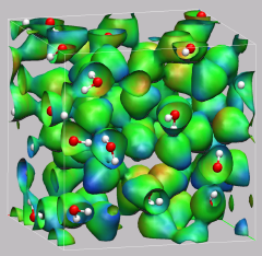
8.2. Hydronium Ion in Bulk Water
9. Exercise: Determination of Dynamic Properties
9.1. Calculation of Vibrational Spectra
9.2. The 'Dragging Effect'
10. Proton Transfer in a Catalytic Triade Model
10.1. Preparing a Model from a Large System
10.2. Equilibration with a Blocked Reaction Path
10.3. Modelling Part of the Reaction Path
10.4. Calculating Electron Structure Properties and Visualizations
11. Credits
12. Downloads
13. File distribution policy
|
|
|
||
|
|||