|
|
|
|
CPMD Tutorial Part 4 |
|
5.3. Geometry Optimization
![]()
5.4. Car-Parrinello Molecular Dynamics
![]()
5.5. Further Job Types
![]()
5.6. How to Use the Tutorial
![]()
![]() Part 3
Part 3
![]() Part 5
Part 5
![]() Start
Start
![]() Contents
Contents
A geometry optimization is not much else than repeated single point calculations, where the positions of the atoms are updated according to the forces acting on them. The required changes in the input file are rather small (5-h2-geoopt.inp):
&CPMD OPTIMIZE GEOMETRY XYZ CONVERGENCE ORBITALS 1.0d-7 CONVERGENCE GEOMETRY 1.0d-4 &END |
We have replaced WAVEFUNCTION with GEOMETRY and added the suboption XYZ to have CPMD write a 'trajectory' of the optimization in a file name GEO_OPT.xyz (so it can be visualized later). Also we specify the convergence parameter for the geometry.
Now again start the CPMD program:
cpmd.x 5-h2-geoopt.inp> 5-h2-geoopt.out |
This run should take a little longer, than the previous one, since we have to do multiple wavefunction optimizations.
OPTIMIZATION OF IONIC POSITIONS [...] CONVERGENCE CRITERIA FOR GEOMETRY OPTIMIZATION: 1.000000E-04 GEOMETRY OPTIMIZATION BY GDIIS/BFGS SIZE OF GDIIS MATRIX: 5 GEOMETRY OPTIMIZATION IS SAVED ON FILE GEO_OPT.xyz EMPIRICAL INITIAL HESSIAN (DISCO PARAMETRISATION) |
As you can see from the first part of the output file (5-h2-geoopt.out), CPMD has recognized the job type, our convergence parameter and the request to write a GEO_OPT.xyz file.
================================================================ = GEOMETRY OPTIMIZATION = ================================================================ NFI GEMAX CNORM ETOT DETOT TCPU EWALD| SUM IN REAL SPACE OVER 1* 1* 1 CELLS 1 3.816E-02 2.886E-03 -1.096898 -1.097E+00 1.28 2 8.628E-03 1.041E-03 -1.130803 -3.391E-02 1.33 [...] 10 1.871E-08 5.247E-09 -1.132460 -8.509E-13 1.43 RESTART INFORMATION WRITTEN ON FILE ./RESTART.1 ATOM COORDINATES GRADIENTS (-FORCES) 1 H 8.2600 7.5589 7.5589 -1.780E-02 9.179E-17 7.909E-17 2 H 6.8578 7.5589 7.5589 1.780E-02 1.596E-16 1.396E-16 **************************************************************** *** TOTAL STEP NR. 10 GEOMETRY STEP NR. 1 *** *** GNMAX= 1.779864E-02 ETOT= -1.132460 *** *** GNORM= 1.027605E-02 DETOT= 0.000E+00 *** *** CNSTR= 0.000000E+00 TCPU= 13.63 *** **************************************************************** 1 5.012E-03 9.718E-04 -1.131471 9.887E-04 1.34 2 4.287E-04 1.613E-04 -1.132846 -1.375E-03 1.35 3 1.489E-04 3.429E-05 -1.132883 -3.659E-05 1.33 |
In the following output you can see, that an almost identical wavefunction optimization takes place. After printing the positions and forces of the atoms, however, you see a small report block and then another wavefunction optimization starts. The numbers for GNMAX, GNORM, and CNSTR stand for the largest absolute component of the force on any atom, average force on the atoms, and the largest absolute component of a constraint force on the atoms respectively.
ATOM COORDINATES GRADIENTS (-FORCES) 1 H 8.2854 7.5589 7.5589 9.965E-05 1.105E-16 9.709E-17 2 H 6.8324 7.5589 7.5589 -9.965E-05 1.835E-16 1.392E-16 **************************************************************** *** TOTAL STEP NR. 36 GEOMETRY STEP NR. 5 *** *** GNMAX= 9.965023E-05 [5.98E-05] ETOT= -1.132896 *** *** GNORM= 5.753309E-05 DETOT= -1.423E-08 *** *** CNSTR= 0.000000E+00 TCPU= 6.76 *** **************************************************************** ================================================================ = END OF GEOMETRY OPTIMIZATION = ================================================================ |
At the end of the geometry optimization, you can see that the forces and the total energy have significantly decreased from their start values as it is to be expected.
Based on the previously calculated electronic structure, we can now also start a 'real' Car-Parrinello calculation. Note that although you can start a CP-MD run from a non-converged wavefunction (e.g. by not restarting from a pre-optimized wavefunction), you will be far away from the Born-Oppenheimer surface, and thus your result will be unphysical.
For the CP-MD job you need a new input file, 6b-h2-md-4au.inp, which should be copied into the same directory, where you started the wavefunction optimization run. If you compare it to the previous input files, you will find, that the only changes are again only in the &CPMD section of the input file.
|
|
The keyword MOLECULAR DYNAMICS CP defines the job type. Furthermore we tell the CPMD program to pick up the previously calculated wavefunction and coordinates from the latest restart file (which is named RESTART.1 by default). MAXSTEP limits the MD to 200 steps and the equations of motion will be solved for a time step of 4 atomic units (~0.1 femtoseconds). The temperature of the system will be initialized to 50K via the TEMPERATURE keyword (note that this is no thermostatting). The keyword TRAJECTORY XYZ will have CPMD write the coordinates additionally to a file TRAJEC.xyz, which can be easily visualized with many molecule viewer programs.
Now start the CPMD program once more:
cpmd.x 6b-h2-md-4au.out> 6b-h2-md-4au.out |
This run should be completed in a few minutes. The output of the CPMD program is now in the file . There also are some more new files (TRAJEC.xyz, TRAJECTORY, ENERGIES), be we'll have a closer look at output file first.
 CAR-PARRINELLO MOLECULAR DYNAMICS

 PATH TO THE RESTART FILES:                                    ./
 RESTART WITH OLD ORBITALS
 RESTART WITH OLD ION POSITIONS
 RESTART WITH LATEST RESTART FILE
 ITERATIVE ORTHOGONALIZATION
    MAXIT:                                                     30
    EPS:                                                 1.00E-06
 MAXIMUM NUMBER OF STEPS:                               200 STEPS
|
The header is unchanged up to the point where the settings from the &CPMD section are printed. As you can see, the program has recognized the RESTART and the MAXSTEP keywords. (NOTE: in the CPMD code atoms are sometimes referred to as ions, which may be sometimes confusing. This is due to the pseudopotential approach, where you integrate the core electrons into the (pseudo)atom which then could be also described as an ion.)
TIME STEP FOR ELECTRONS: 4.0000 TIME STEP FOR IONS: 4.0000 TRAJECTORIES ARE SAVED ON FILE TRAJEC.xyz IS SAVED ON FILE ELECTRON DYNAMICS: THE TEMPERATURE IS NOT CONTROLLED ION DYNAMICS: THE TEMPERATURE IS NOT CONTROLLED |
This part of the output tells us, that the TIMESTEP 4.0 keyword was recognized (the default is 5.0 a.u., cf. the wavefunction output file), that the trajectory will be recorded and that there will be no temperature control, i.e. we will do a microcanonical (NVE-ensemble) simulation.
RV30| WARNING! NO WAVEFUNCTION VELOCITIES RESTART INFORMATION READ ON FILE ./RESTART.1 |
Here we get notified, that the program has read the requested data from the restart file. The warning about the missing wavefunction velocities is to be expected, since they will only be available when the restart was written by a previous Car-Parrinello MD run.
       NFI    EKINC   TEMPP           EKS      ECLASSIC          EHAM         DIS    TCPU
         1  0.00000    49.4      -1.13289      -1.13266      -1.13266   0.207E-05    1.37
         2  0.00000    47.7      -1.13289      -1.13266      -1.13266   0.817E-05    1.36
         3  0.00001    45.7      -1.13288      -1.13267      -1.13266   0.181E-04    1.37
         4  0.00001    43.5      -1.13288      -1.13267      -1.13266   0.314E-04    1.37
         5  0.00002    41.5      -1.13287      -1.13268      -1.13266   0.481E-04    1.37
         6  0.00002    39.8      -1.13287      -1.13268      -1.13266   0.677E-04    1.36
         7  0.00002    38.3      -1.13286      -1.13268      -1.13266   0.901E-04    1.34
         8  0.00002    37.1      -1.13286      -1.13268      -1.13266   0.115E-03    1.38
         9  0.00002    35.9      -1.13285      -1.13268      -1.13266   0.143E-03    1.36
        10  0.00002    34.8      -1.13284      -1.13268      -1.13266   0.173E-03    1.36
        11  0.00002    33.6      -1.13284      -1.13268      -1.13266   0.206E-03    1.39
        12  0.00002    32.4      -1.13283      -1.13267      -1.13266   0.240E-03    1.37
        13  0.00001    31.2      -1.13282      -1.13267      -1.13266   0.277E-03    1.37
        14  0.00001    30.0      -1.13281      -1.13267      -1.13266   0.314E-03    1.37
        15  0.00001    28.9      -1.13281      -1.13267      -1.13266   0.354E-03    1.36
        16  0.00001    27.8      -1.13280      -1.13267      -1.13266   0.394E-03    1.35
        17  0.00001    26.9      -1.13279      -1.13267      -1.13266   0.436E-03    1.37
        18  0.00001    26.1      -1.13279      -1.13267      -1.13266   0.478E-03    1.36
        19  0.00001    25.4      -1.13279      -1.13267      -1.13266   0.521E-03    1.37
        20  0.00001    25.0      -1.13278      -1.13267      -1.13266   0.564E-03    1.38
        21  0.00001    24.8      -1.13278      -1.13267      -1.13266   0.608E-03    1.37
        22  0.00001    24.8      -1.13278      -1.13267      -1.13266   0.652E-03    1.37
        23  0.00001    25.1      -1.13279      -1.13267      -1.13266   0.696E-03    1.36
        24  0.00001    25.5      -1.13279      -1.13267      -1.13266   0.741E-03    1.40
        25  0.00001    26.2      -1.13279      -1.13267      -1.13266   0.786E-03    1.36
       ...
       180  0.00002    43.1      -1.13288      -1.13268      -1.13266   0.321E-01    1.39
       181  0.00002    42.2      -1.13287      -1.13267      -1.13266   0.325E-01    1.36
       182  0.00001    41.1      -1.13287      -1.13267      -1.13266   0.328E-01    1.35
       183  0.00001    39.8      -1.13286      -1.13267      -1.13266   0.331E-01    1.36
       184  0.00001    38.4      -1.13285      -1.13267      -1.13266   0.335E-01    1.37
       185  0.00001    36.8      -1.13284      -1.13267      -1.13266   0.339E-01    1.37
       186  0.00001    35.2      -1.13284      -1.13267      -1.13266   0.342E-01    1.36
       187  0.00001    33.5      -1.13283      -1.13267      -1.13266   0.346E-01    1.37
       188  0.00001    32.0      -1.13282      -1.13267      -1.13266   0.349E-01    1.35
       189  0.00001    30.5      -1.13281      -1.13267      -1.13266   0.353E-01    1.37
       190  0.00001    29.3      -1.13281      -1.13267      -1.13266   0.357E-01    1.37
       191  0.00001    28.2      -1.13280      -1.13267      -1.13266   0.361E-01    1.36
       192  0.00001    27.4      -1.13280      -1.13267      -1.13266   0.365E-01    1.36
       193  0.00001    26.8      -1.13280      -1.13267      -1.13266   0.369E-01    1.35
       194  0.00001    26.4      -1.13279      -1.13267      -1.13266   0.372E-01    1.37
       195  0.00001    26.2      -1.13279      -1.13267      -1.13266   0.376E-01    1.35
       196  0.00001    26.1      -1.13279      -1.13267      -1.13266   0.380E-01    1.36
       197  0.00001    26.3      -1.13279      -1.13267      -1.13266   0.385E-01    1.38
       198  0.00001    26.6      -1.13279      -1.13267      -1.13266   0.389E-01    1.35
       199  0.00001    27.2      -1.13280      -1.13267      -1.13266   0.393E-01    1.36
       200  0.00001    28.0      -1.13280      -1.13267      -1.13266   0.397E-01    1.38
|
After some more output, we already discussed for the wavefunction optimization, this is now part of the energy summary for a Car-Parrinello-MD run.
| The individual columns have the following meaning: | |
|---|---|
| NFI: | Step number (number of finite iterations) |
| EKINC: | (fictitious) kinetic energy of the electronic (sub-)system |
| TEMPP: | Temperature (= kinetic energy / degrees of freedom) for atoms (ions) |
| EKS: | Kohn-Sham Energy, equivalent to the potential energy in classical MD |
| ECLASSIC: | Equivalent to the total energy in a classical MD (ECLASSIC = EHAM - EKINC) |
| EHAM: | total energy, should be conserved |
| DIS: | mean squared displacement of the atoms from the initial coordinates. |
| TCPU: | (CPU) time needed for this step. |
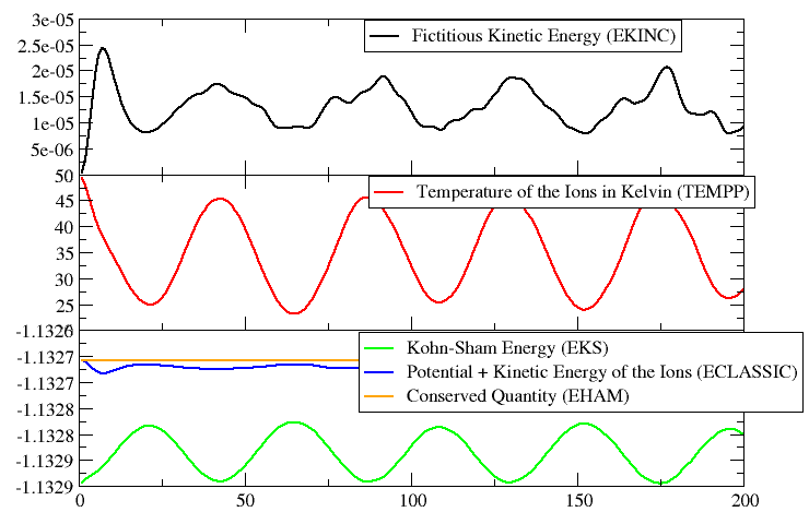 The plot on the left (click on the image for a larger version) shows
the evolution of the various energies during the
simulation. You can see, how a little energy from the ionic system is
transferred to the fictitious electron dynamics (since the temperature
never reaches the initial 50K again) and how this compares to the other
energies: the difference between the orange (EHAM) and the blue
(ECLASSIC) graphs is EKINC, and the difference to the potential energy
(EKS) is kinetic energy in the ionic system.
The plot on the left (click on the image for a larger version) shows
the evolution of the various energies during the
simulation. You can see, how a little energy from the ionic system is
transferred to the fictitious electron dynamics (since the temperature
never reaches the initial 50K again) and how this compares to the other
energies: the difference between the orange (EHAM) and the blue
(ECLASSIC) graphs is EKINC, and the difference to the potential energy
(EKS) is kinetic energy in the ionic system.
At the end of the geometry optimization the hydrogen molecule was in the minimum of its potential. Now after starting the MD, we see that the initial kinetic energy added to the system is slowly converted into potential energy (cf. EKS) as the bond is elongated. After a while the molecule has reached the maximal elongation and the potential energy is converted back into kinetic energy (i.e. the temperature rises again). So we have a regular oscillation of the hydrogen molecule. You can also see, that a little bit of energy is transferred into the fictitious dynamic of the electronic degrees of freedom. For a meaningful Car-Parrinello MD this value has to be (and stay) very small (although for larger systems with more electrons, the absolute value of EKINC will be larger).
****************************************************************
* AVERAGED QUANTITIES *
****************************************************************
MEAN VALUE +/- RMS DEVIATION
|
Finally we get a summary of some averages and root mean squared deviations for some of the monitored quantities. This is quite useful to detect unwanted energy drifts or too large fluctuations in the simulation.
If you want to visualize the motion of the hydrogen atoms, you can load the file TRAJEC.xyz directly into a molecular visualization program like gopenmol, molden, molekel, vmd or xmol.
KOHN-SHAM ENERGIES PROPERTIES LINEAR RESPONSE VIBRATIONAL ANALYSIS ORBITAL HARDNESS ELECTRONIC SPECTRA |
The previous pages are a short introduction into the 'mechanics' of running a CPMD job, usually something that would be explained to you in person by an advisor during the course of your your first steps with CPMD. Since we don't have this way of communication here, it is suggested, you start the tutorial pages from here and then go back and forth in whatever way you need it.
To further help you, you can also browse not only the full directory tree with the collected input files, but also a similar directory with collected reference outputs and a directory with collected additional material. Although there is no harm in having a peek there, if you are 'stuck', but as usual, the learning experience will be best, if you try hard to delay this as long as possible. ;-) See the Downloads Section for downloadable archives with the complete inputs or outputs.
Full Table of Contents
![]()
1. Introduction
1.1. Development Notice
1.2. Notes
1.3. Recent Changes
1.4. Citation / Bookmark
2. Table of Contents
3. Preparation and Installation Issues
3.1. Compiling CPMD
3.2. Running CPMD
3.3. Running cpmd2cube
4. The Theory: Some Fundamental Infos and Useful Literature
5. The Basics: Running CPMD, Input and Output Formats
5.1. Wavefunction Optimization: a) Input File Format
5.2. Wavefunction Optimization: b) Output File Format
5.3. Geometry Optimization
5.4. Car-Parrinello Molecular Dynamics
5.5. Further Job Types
5.6. How to Use the Tutorial
6. Exercise: Electron Structure and Geometry Optimization
6.1. Hydrogen Molecule
6.2. Water Molecule
6.3. Ammonia Molecule
7. Exercise: Car-Parrinello Molecular Dynamics
7.1. Hydrogen Molecule
7.2. Ammonia Molecule in Gas Phase
7.3. Glycine Molecule in Gas Phase
7.4. Glycine with Thermostats
8. Exercise: Bulk Systems
8.1. Bulk Silicon
8.2. Hydronium Ion in Bulk Water
9. Exercise: Determination of Dynamic Properties
9.1. Calculation of Vibrational Spectra
9.2. The 'Dragging Effect'
10. Proton Transfer in a Catalytic Triade Model
10.1. Preparing a Model from a Large System
10.2. Equilibration with a Blocked Reaction Path
10.3. Modelling Part of the Reaction Path
10.4. Calculating Electron Structure Properties and Visualizations
11. Credits
12. Downloads
13. File distribution policy
|
|
|
||
|
|||